1D GPE

1D GPE#

The GPE in 1D with constant potential is integrable. Here we explain what this means.

We start by assuming we have a solution \(\psi(x, t)\) to the GPE:

\[\begin{gather*} \I\hbar\dot{\psi} = \frac{-\hbar^2}{2m}\psi'' + g\abs{\psi}^2\psi. \end{gather*}\]

Show that the eigenvalues of the following Lax operator do not change in time:

\[\begin{gather*} \op{L} = \frac{\hbar}{2m} \begin{pmatrix} \I\partial_{x} & -\I\sqrt{k_c}\psi^*\\ \I\sqrt{k_c}\psi & -\I\partial_{x} \end{pmatrix}, \qquad k_c = \frac{mg}{\hbar^2},\\ \op{L}\phi = \phi\lambda, \qquad \lambda_{,t} = 0. \end{gather*}\]

The spectrum allows one to characterize the state \(\psi(x, t)\) in terms of non-linear excitations with discrete eigenvalues correspond to solitons, and a continuum. The eigenvalues \(\lambda\) are the velocities of the corresponding excitations.

One often sees associated with the Lax operator \(\op{L}\), another operator \(\op{A}\) which effects a time-derivative. Together these are referred to as a Lax pair and they have the following property obtained by differentiating the eigenvalue equation:

\[\begin{gather*} \op{L}\phi = \phi\lambda, \qquad \op{A}\phi = \phi_{,t},\qquad \op{L}_{,t} + [\op{L}, \op{A}] = 0. \end{gather*}\]

Note

To simplify the algebra, we choose units where \(2m = \hbar = m\!\abs{g} = 1\), so that the GPE and Lax operator assume the following dimensionless forms:

\[\begin{gather*} \I\dot{\psi} = -\partial_x^2\psi + 2ℵ(\abs{\psi}^2 - \rho^2)\psi, \qquad \op{L}^\dagger = \begin{pmatrix} \I\partial_{x} & -\I\sqrt{ℵ}\psi^*\\ \I\sqrt{ℵ}\psi & -\I\partial_{x} \end{pmatrix}, \end{gather*}\]

with \(ℵ \pm 1\). This matches the notation of [Faddeev and Takhtajan, 1987]. Following their approach, we included a constant background density \(\rho^2 = \psi_0^2\) here which allows use to use time-independent twisted boundary conditions if needed.

Repulsive interactions \(g>0\) have \(ℵ = 1\) which is often referred to as de-focusing. Attractive interactions \(g<0\) have \(ℵ = -1\) which is referred to as focusing.

from sympy import *
hbar = 1
m = S(1)/2
g = S(1)/m
t, x, psi0, theta = var('t, x, psi_0, theta', positive=True, real=True)
n = psi0**2
c = sqrt(g*n/m)
v = c*cos(theta)
u = c*sin(theta)
l = hbar/m/u
n = psi0**2
mu = g*n
psi = psi0*exp(mu*t/I/hbar)*(I*v/c + u/c*tanh((x-v*t)/l))
psic = psi.conjugate()
eq = -hbar**2*psi.diff(x, x)/2/m + g*(psi*psic)*psi - I*hbar*psi.diff(t)
eq.simplify()

\[\displaystyle 0\]

Solitons

Consider an eigenstate in the de-focusing case \(ℵ = 1\). It is well known that this theory supports soliton solutions

\[\begin{gather*} c = \sqrt{\frac{gn}{m}}, \qquad u = \sqrt{1 - \frac{v^2}{c^2}}, \qquad l = \frac{\hbar}{mu}\\ \psi(x,t) = \psi_0e^{\mu t /\I\hbar}\Biggl( \I \frac{v}{c} + \frac{u}{c}\tanh\bigl(\frac{x-vt}{l}\bigr) \Biggr),\\ \end{gather*}\]

\[\begin{gather*} c = \sqrt{\frac{g\psi_0^2}{m}}\\ u = \frac{\sqrt{c^2-v^2}}{c}, \qquad l = \frac{\hbar}{mu}\\ \psi(x) = \psi_0\Bigl(\I \frac{v}{c} + \frac{\sqrt{c^2-v^2}}{c}\tanh\frac{x}{l}\Bigr) \end{gather*}\]

which whose field is asymptotically flat

\[\begin{gather*} \psi(x\rightarrow \infty) = -\psi(x\rightarrow -\infty) = \psi_0. \end{gather*}\]

Grey solitons with velocity \(v = \lambda\) should satisfy this equation:

\[\begin{gather*} \I\phi_1' - \I\psi^*\phi_2 = v \phi_1, \qquad -\I\phi_2' + \I\psi\phi_1 = v \phi_2. \end{gather*}\]

Solving for \(\phi_1\) and inserting this, we have

\[\begin{gather*} \phi_1 = \frac{v \phi_2 + \I\phi_2'}{\I\psi},\\ \I\partial_x\frac{v \phi_2 + \I\phi_2'}{\I\psi} - \I\psi^*\phi_2 = v \frac{v \phi_2 + \I\phi_2'}{\I\psi} \end{gather*}\]

Details

We start with some formalism from [Ablowitz and Clarkson, 1991]. The start with the following scattering problem expressed as two linear equations:

\[\begin{gather*} v_{,x} = \mat{X}v, \qquad v_{,t} = \mat{T}v. \end{gather*}\]

Consistency of mixed partials \(v_{,xt} = v_{,tx}\) requires

\[\begin{gather*} \mat{X}_{,t} - \mat{T}_{,x} + [\mat{X}, \mat{T}] = \mat{0}. \end{gather*}\]

The GPE comes from a 2×2 system, which they parameterize as

\[\begin{gather*} \mat{X} = \begin{pmatrix} -\I k & q\\ r & \I k \end{pmatrix}, \qquad \mat{T} = \begin{pmatrix} A & B\\ C & D \end{pmatrix}, \end{gather*}\]

where \(q\), \(r\), \(A\), \(B\), \(C\), and \(D\) are functions of \((x,t;k)\). They also assume that \(k\) is time-independent: \(\dot{k} = 0\).

We can turn \(v_{,x} = \mat{X}v\) into the Lax eigenvalue equation by isolating the eigenvalue:

\[\begin{gather*} \mat{X} = -\I \mat{\sigma}_{z} k + \mat{M}, \qquad \mat{M} = \begin{pmatrix} 0 & q\\ r & 0 \end{pmatrix}. \end{gather*}\]

From \(\mat{X}\) we can find a differentiation operator:

\[\begin{gather*} v_{,x} = \partial_x v = \mat{X}v = (-\I \mat{\sigma}_{z} k + \mat{M})v\\ \I\mat{\sigma}_z\partial_x v = (k + \I\mat{\sigma}_z\mat{M})v,\\ (\I\mat{\sigma}_z\partial_x - \I\mat{\sigma}_z\mat{M}) v = kv. \end{gather*}\]

Hence, we can identify \(k \equiv \lambda\), \(v \equiv \phi\) , and

\[\begin{gather*} \op{L} = \I\mat{\sigma}_z\partial_x - \I\mat{\sigma}_z\mat{M} = \begin{pmatrix} \I\partial_x & -\I q\\ \I r & -\I\partial_x \end{pmatrix},\qquad \op{A} = \mat{T}. \end{gather*}\]

We now need to find matrices \(\mat{X}\) and \(\mat{T}\) whose consistency condition is equivalent to the GPE. They give a solution with a different sign convention, so we instead follow the example in [Faddeev and Takhtajan, 1987], identifying

\[\begin{gather*} \begin{pmatrix} v\\ \mat{X}\\ \mat{T}\\ k \end{pmatrix} \equiv \begin{pmatrix} F\\ \mat{U}\\ \mat{V}\\ \frac{\lambda}{2} \end{pmatrix}. \end{gather*}\]

To simplify the algebra, we choose units where \(2m = \hbar = mg = 1\), so that the GPE and Lax operator assume the following dimensionless forms:

\[\begin{gather*} \I\dot{\psi} = -\partial_x^2\psi + 2ℵ(\abs{\psi}^2 - \rho^2)\psi, \qquad \op{L}^\dagger = \begin{pmatrix} \I\partial_{x} & -\I\sqrt{ℵ}\psi^*\\ \I\sqrt{ℵ}\psi & -\I\partial_{x} \end{pmatrix}, \end{gather*}\]

with \(ℵ = \pm 1\). This follows the notation of [Faddeev and Takhtajan, 1987] which contains the best presentation of this material I have yet found. Following their presentation, we have included a constant background density \(\rho^2\) here which allows use to use time-independent twisted boundary conditions if needed.

Working with the Lax operator is not so easy because of the derivatives: i.e. you must be careful with commutators \([\partial_x, f] = f_{,x}\). Instead, [Faddeev and Takhtajan, 1987] replaces this with a zero-curvature representation:

\[\begin{gather*} \mat{U}_{,t} - \mat{V}_{,x} + [\mat{U}, \mat{V}] = 0, \qquad F_{,x} = \mat{U}F, \qquad F_{,t} = \mat{V}F. \end{gather*}\]

The NS model follows from the compatibility conditions (zero-curvature conditions):

\[\begin{gather*} \I\dot{ψ} = -ψ_{,xx} + 2ℵ(\abs{ψ}^2 - \rho^2),\tag{1.5}\\ \mat{U} = \mat{U}_0 + \lambda \mat{U}_1, \tag{2.3}\\ \mat{V} = \mat{V}_0 + \lambda \mat{V}_1 + \lambda^2\mat{V}_2, \tag{2.6}\\ \mat{U}_0 = \sqrt{ℵ}(ψ^*\mat{σ}_{+} + ψ\mat{σ}_{-}), \tag{2.4}\\ \mat{U}_1 = \frac{\mat{σ}_{z}}{2\I}, \tag{2.5}\\ \mat{V}_0 = \I ℵ (\abs{ψ}^2 - \rho^2)\mat{σ}_{z} - \I\sqrt{ℵ} (ψ^*_{,x}\mat{σ}_+ - ψ_{,x}\mat{σ}_-), \tag{2.7}\\ \mat{V}_1 = -\mat{U}_0, \qquad \mat{V}_2 = -\mat{U}_1, \tag{2.8}\\ \mat{U}_{,t} - \mat{V}_{,x} + [\mat{U},\mat{V}] = \mat{0}, \tag{2.10}\\ \mat{U} = \begin{pmatrix} \frac{\lambda}{2\I} & \sqrt{ℵ}ψ^* \\ \sqrt{ℵ}ψ & \frac{-\lambda}{2\I} \end{pmatrix},\\ \mat{V} = \begin{pmatrix} \I ℵ (\abs{ψ}^2 - ρ^2) - \frac{\lambda^2}{2\I} & \I\sqrt{ℵ}ψ^*_{,x} - \lambda\sqrt{ℵ}ψ^*\\ - \I\sqrt{ℵ}ψ_{,x} - \lambda\sqrt{ℵ}ψ & -\I ℵ (\abs{ψ}^2 - ρ^2) + \frac{\lambda^2}{2\I} \end{pmatrix}. \end{gather*}\]

The geometric interpretation is that \(\mat{U}(x, t;\lambda)\) and \(\mat{V}(x, t;\lambda)\) are local connection coefficients in the trivial vector bundle \(\mathbb{R}^2\times \mathbb{C}^2\) where \(F(x, t;\lambda):\quad \mathbb{R}^2 \mapsto \mathbb{C}^2\). The compatibility condition is equivalent to the \((\mat{U}, \mat{V})\)-connection having zero curvature. This system has the gauge transformation

\[\begin{align*} F &\rightarrow \mat{G}F, \\ \mat{U} &\rightarrow \mat{G}_{,x}\mat{G}^{-1} + \mat{G}\mat{U}\mat{G}^{-1},\\ \mat{V} &\rightarrow \mat{G}_{,t}\mat{G}^{-1} + \mat{G}\mat{V}\mat{G}^{-1}. \end{align*}\]

The zero-curvature conditions are related to the Lax operator of the inverse-scattering method (ISM) using the identity \(\mat{σ}_{z}\mat{σ}_{\pm} = \pm \mat{σ}_{\pm}\) and applying \(\I\mat{σ}_{z}\) to \(F_{,x} - \mat{U}F = 0\):

\[\begin{gather*} \overbrace{\I\mat{σ}_z\left(\pdiff{}{x} - \mat{U}\right)}^{\op{L} - \frac{\lambda}{2}}F = 0, \qquad \op{L}F = \frac{\lambda}{2}F,\\ \I\mat{σ}_z\mat{U} = \I\sqrt{ℵ}(ψ^*\mat{σ}_+ - ψ\mat{σ}_-) + \frac{\lambda}{2},\\ \begin{aligned} \op{L} &= \I\mat{σ}_{z}\;\!\pdiff{}{x} - \I\mat{σ}_{z}\mat{U} + \frac{\lambda}{2}\\ &= \I\mat{σ}_{z}\;\!\pdiff{}{x} - \I\sqrt{ℵ}(ψ^*\mat{σ}_+ - ψ\mat{σ}_-) = \begin{pmatrix} \I \partial_x & -\I\sqrt{ℵ}ψ^*\\ \I\sqrt{ℵ}ψ & - \I \partial_x \end{pmatrix}. \end{aligned} \end{gather*}\]

This is self-adjoint for the de-focusing case \(ℵ > 0\) with a corresponding real spectrum \(\lambda/2\).

To Do: This does not quite work. Why? To check that \(\op{L}\) and \(\op{A} = \mat{V}\) form a Lax pair, we compute

\[\begin{gather*} \op{L}_{,t} = -\I\mat{σ}_{z}\mat{U}_{,t}\\ [\op{L}, \mat{V}] = [\I\mat{σ}_{z} \partial_x - \I\mat{σ}_{z}\mat{U}, \mat{V}] = [\I\mat{σ}_{z} \partial_x, \mat{V}] - [\I\mat{σ}_{z}\mat{U}, \mat{V}]\\ = \I\mat{σ}_{z}[\partial_x, \mat{V}] + [\I\mat{σ}_{z}, \mat{V}]\partial_x - \I\mat{σ}_{z}[\mat{U}, \mat{V}] - [\I\mat{σ}_{z}, \mat{V}]\mat{U}\\ = \I\mat{σ}_{z}\Bigl([\partial_x, \mat{V}] - [\mat{U}, \mat{V}] \Bigr) + [\I\mat{σ}_{z}, \mat{V}](\partial_x - \mat{U})\\ = \I\mat{σ}_{z}\Bigl(\mat{V}_{,x} - [\mat{U}, \mat{V}]\Bigr) + [\I\mat{σ}_{z}, \mat{V}](-\I\mat{σ}_{z})\op{L}\\ = \I\mat{σ}_{z}\mat{U}_{,t} - [\I\mat{σ}_{z}, \mat{V}]\I\mat{σ}_{z}\op{L}. \end{gather*}\]

Thus

\[\begin{gather*} \op{L}_{,t} + [\op{L}, \mat{V}] = - [\I\mat{σ}_{z}, \mat{V}]\I\mat{σ}_{z}\op{L}. \end{gather*}\]

# Here we show that the formulae in Faddeev:1987 work
import IPython.display
import sympy
from sympy import var, Function, Symbol, Matrix, I, Eq, S, sqrt
x, t, lam, g, rho = var('x, t, lambda, aleph, rho')
psi = Function('psi')(x, t)
psic = psi.conjugate()
Sp = Matrix([[0, 1], 
             [0, 0]])
Sm = Sp.T
Sz = Matrix([[1, 0], 
             [0, -1]])

# To display things nicely, we introduce some subsitutions
psi_ = Symbol('psi')
psi_x_ = Symbol(r'\psi_{,x}')
psi_xx_ = Symbol(r'\psi_{,xx}')
psic_ = Symbol(r'\bar{\psi}')
psic_x_ = Symbol(r'\bar{\psi}_{,x}')
psic_xx_ = Symbol(r'\bar{\psi}_{,xx}')
ss_ = {
  psi.diff(x,x): psi_xx_,
  psic.diff(x,x): psic_xx_,
  psi.diff(x): psi_x_,
  psic.diff(x): psic_x_,
  psi: psi_, 
  psic: psic_,
}

def show_eq(a, b):
    display(IPython.display.Latex(f"{a} = {sympy.latex(b.subs(ss_))}"))

# This is the GPE or NLSEQ (1.5)
ss = {psi.diff(t): (-psi.diff(x,x) + 2*g*(psic*psi - rho**2)*psi)/I,
      psic.diff(t): -(-psic.diff(x,x) + 2*g*(psic*psi - rho**2)*psic)/I}

# Here are the forumulae from Faddeev:1987
U0 = sqrt(g)*(psic*Sp + psi*Sm)    # (2.4)
U1 = Sz/2/I                        # (2.5)
V0 = (I*g*(psi*psic - rho**2)*Sz   # (2.7 + 2.11) 
     - I*sqrt(g)*(psic.diff(x)*Sp - psi.diff(x)*Sm))
V1, V2 = -U0, -U1                  # (2.8)
U = U0 + lam*U1                    # (2.3)
V = V0 + lam*V1 + lam**2*V2        # (2.6)

res = U.diff(t).subs(ss) - V.diff(x) + U@V - V@U  # (2.10)
res.simplify()
assert res == Matrix([[0,0], [0,0]])
    
show_eq("U", U)
show_eq("V", V)

res1 = sympy.simplify(U.diff(t))
res2 = sympy.simplify(V.diff(x) - U@V + V@U)

display(Eq(
  (sympy.I * res1 @ Sz / sympy.sqrt(g)).subs(ss_),
  (sympy.I * res2 @ Sz / sympy.sqrt(g)).subs(ss_)))
  
# Remainder term from Lax pair... this is not zero... WHY?
display(((Sz@V - V@Sz)@Sz).subs(ss_))

\[\begin{split}U = \left[\begin{matrix}- \frac{i \lambda}{2} & \bar{\psi} \sqrt{\aleph}\\\sqrt{\aleph} \psi & \frac{i \lambda}{2}\end{matrix}\right]\end{split}\]

\[\begin{split}V = \left[\begin{matrix}i \aleph \left(\bar{\psi} \psi - \rho^{2}\right) + \frac{i \lambda^{2}}{2} & - \bar{\psi} \sqrt{\aleph} \lambda - i \bar{\psi}_{,x} \sqrt{\aleph}\\i \psi_{,x} \sqrt{\aleph} - \sqrt{\aleph} \lambda \psi & - i \aleph \left(\bar{\psi} \psi - \rho^{2}\right) - \frac{i \lambda^{2}}{2}\end{matrix}\right]\end{split}\]

\[\begin{split}\displaystyle \left[\begin{matrix}0 & - i \frac{d}{d t} \bar{\psi}\\i \frac{d}{d t} \psi & 0\end{matrix}\right] = \left[\begin{matrix}0 & 2 \bar{\psi}^{2} \aleph \psi - 2 \bar{\psi} \aleph \rho^{2} - \bar{\psi}_{,xx}\\2 \bar{\psi} \aleph \psi^{2} - \psi_{,xx} - 2 \aleph \psi \rho^{2} & 0\end{matrix}\right]\end{split}\]

\[\begin{split}\displaystyle \left[\begin{matrix}0 & 2 \bar{\psi} \sqrt{\aleph} \lambda + 2 i \bar{\psi}_{,x} \sqrt{\aleph}\\- 2 i \psi_{,x} \sqrt{\aleph} + 2 \sqrt{\aleph} \lambda \psi & 0\end{matrix}\right]\end{split}\]

\[q_{,t} = \frac{a \left(2 q^{2} r - q_{,xx}\right)}{2}\]

\[r_{,t} = \frac{a \left(- 2 q r^{2} + r_{,xx}\right)}{2}\]

\[\begin{split}\displaystyle \left[\begin{matrix}i \left(2 k^{2} - q s \overline{q}\right) & - 2 k q - i q_{,x}\\s \left(- i \bar{q}_{,x} + 2 k \overline{q}\right) & i \left(- 2 k^{2} + q s \overline{q}\right)\end{matrix}\right]\end{split}\]

\[\begin{split}X = \left[\begin{matrix}- i k & q\\s \overline{q} & i k\end{matrix}\right]\end{split}\]

\[\begin{split}T = \left[\begin{matrix}i \left(- 2 k^{2} - q s \overline{q}\right) & 2 k q + i q_{,x}\\s \left(- i \bar{q}_{,x} + 2 k \overline{q}\right) & i \left(2 k^{2} + q s \overline{q}\right)\end{matrix}\right]\end{split}\]

\[i q_{,t} = 2 q^{2} s \overline{q} - q_{,xx}\]

\[i \bar{q}_{,t} = \bar{q}_{,xx} - 2 q s \overline{q}^{2}\]

\[i q_{,t} = - 8 k^{2} q - 2 q^{2} s \overline{q} - q_{,xx}\]

\[i \bar{q}_{,t} = \bar{q}_{,xx} s + 4 k^{2} s \overline{q} + 4 k^{2} \overline{q} + 2 q s \overline{q}^{2}\]

\[i q_{,t} = 2 q^{2} s \overline{q} + q_{,xx}\]

\[i \bar{q}_{,t} = - \bar{q}_{,xx} - 2 q s \overline{q}^{2}\]

# Testing (1.9.2)
a, x, t = symbols('a, x, t', real=True)
k = symbols('k')
u = Function('u')(x, t)
f1, f2 = Function('f_1')(x, t), Function('f_2')(x, t)
f = Matrix([[f1], [f2]])
uc = u.conjugate()

L0 = Matrix([[0, uc], [u, 0]])
L1 = I*Matrix([[1+k, 0], [0, 1-k]])
M0 = Matrix([[-I*u*uc/(1+k), uc.diff(x)],
             [-u.diff(x), I*u*uc/(1-k)]])
M2 = I*k*Matrix([[1, 0], [0, 1]])

def apply(L, f):
    L0, L1, L2 = L
    return L0 @ f + L1 @ f.diff(x) + L2 @ f.diff(x, x)

L = [L0, L1, 0*M2]
M = [M0, 0*M2, M2]
Lt = [L0.diff(t), L1.diff(t), 0*M2]
res = apply(Lt, f) + apply(L, apply(M, f)) - apply(M, apply(L, f))
res = simplify(res)

def simp(expr):
    expr = simplify(expr)
    u_ = Symbol('u')
    uc_ = u_.conjugate()
    ss_ = {
        uc.diff(x,x): Symbol(r'\bar{u}_{,xx}'),
        uc.diff(x): Symbol(r'\bar{u}_{,x}'),
        uc.diff(t): Symbol(r'\bar{u}_{,t}'),
        uc: uc_,
        u.diff(x,x): Symbol(r'u_{,xx}'),
        u.diff(x): Symbol(r'u_{,x}'),
        u.diff(t): Symbol(r'u_{,t}'),
        u: u_, 
    }
    return expr.subs(ss_)

simp(solve(res[1], u.diff(t))[0])

\[\displaystyle \frac{i \left(k^{2} u_{,xx} - 2 u^{2} \overline{u} - u_{,xx}\right)}{k^{2} - 1}\]

[Ablowitz and Clarkson, 1991]

In the preceding code, we check that the compatibility condition

\[\begin{gather*} \mat{X}_{,t} - \mat{T}_{,x} + [\mat{X}, \mat{T}] = 0, \tag{1.9.7} \end{gather*}\]

with the following:

\[\begin{gather*} \mat{X} = \begin{pmatrix} - \I k & q\\ r & \I k \end{pmatrix}, \qquad \mat{T} = \begin{pmatrix} A & B\\ C & D \end{pmatrix}, \tag{1.9.10}\\ A = ak^2 + \tfrac{1}{2}arq\\ B = \I a q k - \tfrac{1}{2}aq_{,x}\\ C = \I a r k + \tfrac{1}{2}ar_{,x}\\ D = -A\\ \end{gather*}\]

yields the following NLSEQ:

\[\begin{align*} q_{,t} &= aq^2 r - \tfrac{1}{2}aq_{,xx}, \tag{1.9.17a}\\ r_{,t} &= -aq r^2 + \tfrac{1}{2}ar_{,xx}. \tag{1.9.17b}. \end{align*}\]

Setting \(r = \pm q^*\) we have

\[\begin{align*} \I q_{,t} &= \pm \I aq^2q^* - \tfrac{1}{2} \I aq_{,xx},\\ -\I q^*_{,t} &= \pm \I aq(q^*)^2 - \tfrac{1}{2}\I aq^*_{,xx}. \end{align*}\]

Thus, we can reproduce the GPE by setting \(\I a = 2\):

\[\begin{align*} \I q_{,t} &= - q_{,xx} \pm 2 q^2q^*. \end{align*}\]

[Ablowitz and Clarkson, 1991] do something slightly different. They set \(a = 2\I\) to get

\[\begin{gather*} \I q_{,t} = q_{,xx} \pm 2q^2q^*.\tag{1.9.18} \end{gather*}\]

Note, however, that the direct formulae have sign errors. The left column is from [Ablowitz and Clarkson, 1991]. The right column is obtained with \(a = 2\I\) and works.

\[\begin{align*} A &= 2\I k^2 \pm \I q q^* &&\rightarrow & A &= 2\I k^2 \mp \I q q^*, \tag{1.9.19a}\\ B &= 2qk + \I q_{,x} && \rightarrow & B &= -2qk - \I q_{,x}, \tag{1.9.19b}\\ C &= \mp 2 q^* k \pm\I q^*_{,x} &&\rightarrow & C &= \pm 2 q^* k \mp \I q^*_{,x},\tag{1.9.19c}\\ r &= -q^* &&\rightarrow & r &= \mp q^*, \tag{inline} \end{align*}\]

Their notation is equivalent to [Faddeev and Takhtajan, 1987] if we identify

\[\begin{gather*} \begin{pmatrix} v\\ \mat{X}\\ \mat{T}\\ k \end{pmatrix} \equiv \begin{pmatrix} F\\ \mat{U}\\ \mat{V}\\ \frac{\lambda}{2} \end{pmatrix}. \end{gather*}\]

Remarks:

Why do we need opposite signs along the diagonal? It would be nice to have an interpretation that the \(k\) is just the wave-vector, so why do we need the \(\mat{\sigma}_z\)? Probably due to time-reversal or something?
They note that any \(x\)-derivatives in the equation for \(v_{,t}\) can be eliminated by using \(v_{,x} = \mat{X}v\).
If \(r=-1\), we have the time-independent Schrödinger equation:

\[\begin{gather*} v_{1,x} = -\I k v_1 + qv_2, \qquad v_{2,x} = \I k v_2 - v_1, \end{gather*}\]

hence, eliminating \(v_1 = \I k v_2 - v_{2,x}\) we have

\[\begin{gather*} \I k v_{2,x} - v_{2,xx} = -\I k (\I k v_2 - v_{2,x}) + qv_2\\ v_{2,xx} + (k^2 + q)v_2 = 0. \end{gather*}\]

This is the time-independent Schrödinger equation in units where \(\hbar^2 = 2m =1\) with

\[\begin{gather*} k^2 = E, \qquad q = -V(x, t), \qquad v = \begin{pmatrix} \I k^2 \psi(x, t) - \psi_{,x}(x, t)\\ \psi(x, t) \end{pmatrix}. \end{gather*}\]
To relate this to the Lax pair

\[\begin{gather*} \op{L}\phi = \phi \lambda, \qquad \phi_{,t} = \op{A}\phi, \end{gather*}\]

we note that

\[\begin{gather*} \mat{X} = -\I \mat{\sigma}_{z} k + \mat{M}, \qquad \mat{M} = \begin{pmatrix} 0 & q\\ r & 0 \end{pmatrix}. \end{gather*}\]

Hence:

\[\begin{gather*} v_{,x} = \partial_x v = \mat{X}v = (-\I \mat{\sigma}_{z} k + \mat{M})v\\ \I\mat{\sigma}_z\partial_x v = (k + \I\mat{\sigma}_z\mat{M})v,\\ (\I\mat{\sigma}_z\partial_x - \I\mat{\sigma}_z\mat{M}) v = kv. \end{gather*}\]

Hence, we can identify \(k \equiv \lambda\), \(v \equiv \phi\) , and

\[\begin{gather*} \op{L} = \I\mat{\sigma}_z\partial_x - \I\mat{\sigma}_z\mat{M} = \begin{pmatrix} \I\partial_x & -\I q\\ \I r & -\I\partial_x \end{pmatrix},\qquad \op{A} = \mat{T}. \end{gather*}\]

Since \(v_{,xt} = v_{,tx}\) is consistent, differentiating the Lax equation and using \(\dot{\lambda} = 0\) gives the consistency condition

\[\begin{gather*} \op{L}_{,t} + [\op{L}, \op{A}] = 0. \end{gather*}\]

I find it hard to show this explicitly in general.

[Osborne, 2010]

Here they have

\[\begin{gather*} L\phi = \phi\lambda, \qquad \phi_{,t} = A\phi, \qquad \dot{L} + [L, A] = 0, \\ L = \begin{pmatrix} \I\partial_x & u\\ - u^* & -\I\partial_x \end{pmatrix}, \qquad A = \begin{pmatrix} \I \abs{u}^2 - 2\I \lambda^2 & -u_{,x} + 2\I \lambda u\\ -u_{,x}^* + 2\I \lambda u^* & -\I \abs{u}^2 + 2\I \lambda^2 \end{pmatrix}. \end{gather*}\]

Note that \(L\) is not hermitian. This is strange.

Proceeding as per [Ablowitz and Clarkson, 1991], we look for a system

\[\begin{gather*} v_{,x} = \mat{X}v, \qquad v_{,t} = \mat{T}v. \end{gather*}\]

If we take \(v = \phi\), then \(\mat{T} = \mat{A}\). To find \(\mat{X}\) note that

\[\begin{gather*} \mat{1}\partial_{x} = -\I\mat{\sigma}_{z}(\mat{L} - \mat{M}),\\ \mat{M} = \begin{pmatrix} 0 & u\\ -u^* & 0 \end{pmatrix},\\ v_{,x} = -\I\mat{\sigma}_{z}(\mat{L} - \mat{M})v = -\I\mat{\sigma}_{z}(\lambda - \mat{M})v. \end{gather*}\]

Hence

\[\begin{gather*} \mat{X} = -\I\mat{\sigma}_{z}\lambda +\I\mat{\sigma}_{z}\mat{M} = \begin{pmatrix} -\I \lambda & \I u\\ \I u^* & \I \lambda \end{pmatrix}. \end{gather*}\]

We note that this matches the formulation in [Faddeev and Takhtajan, 1987] for \(\mat{U}\) if we take \(\lambda \rightarrow \lambda /2\) and \(u \rightarrow \psi^*\), and \(ℵ=1\):

\[\begin{align*} \mat{X} \equiv \mat{U} &= \begin{pmatrix} \frac{\lambda}{2\I} & \I \psi^*\\ \I \psi & -\frac{\lambda}{2\I} \end{pmatrix},\\ \mat{A} \equiv \mat{T} \equiv \mat{V} &= \begin{pmatrix} \I \abs{\psi}^2 + \tfrac{\lambda^2}{2\I} & -\psi^*_{,x} + \I \lambda \psi^*\\ -\psi_{,x} + \I \lambda \psi & -\I \abs{\psi}^2 - \frac{\lambda^2}{2\I}\I \end{pmatrix}. \end{align*}\]

This second matrix does not match, however. [Faddeev and Takhtajan, 1987] has

\[\begin{gather*} \mat{V} = \begin{pmatrix} \I \abs{ψ}^2 - \frac{\lambda^2}{2\I} & -\I ψ^*_{,x} - \lambda ψ^*\\ \I ψ_{,x} - \lambda ψ & -\I \abs{ψ}^2 + \frac{\lambda^2}{2\I} \end{pmatrix} \end{gather*}\]

which I have checked above. They do not seem to use \(\op{A}\) in [Osborne, 2010], so perhaps this error was overlooked or perhaps it is gauge equivalent – I have not checked yet.

#:tags: [hide-input]

# Test of Osbourne:2010.  It seems there is an error.
x, t, lam, g, rho = var('x, t, lambda, aleph, rho')
g = 1
rho = 0

U0 = sympy.sqrt(g)*(psic*Sp + psi*Sm)
U1 = Sz/2/I
U = U0 + lam*U1
V = Matrix(
    [[I*psi*psic - lam**2/2/I, -psic.diff(x) + I*lam*psic], 
     [-psi.diff(x) + I*lam*psi, -I*psi*psic + lam**2/2/I]])

# From Faddeev
V_ = Matrix(
    [[I*psi*psic - lam**2/2/I, -I*psic.diff(x) - lam*psic], 
     [I*psi.diff(x) - lam*psi, -I*psi*psic + lam**2/2/I]])

ss = {psi.diff(t): (-psi.diff(x,x) + 2*g*(psic*psi - rho**2)*psi)/I,
      psic.diff(t): -(-psic.diff(x,x) + 2*g*(psic*psi - rho**2)*psic)/I}
res = U.diff(t).subs(ss) - V.diff(x) + U@V - V@U

res.simplify()
display(V.subs(ss_))
display(res.subs(ss_))
assert res == Matrix([[0,0], [0,0]])

\[\begin{split}\displaystyle \left[\begin{matrix}\frac{i \lambda^{2}}{2} + i \psi{\left(x,t \right)} \overline{\psi{\left(x,t \right)}} & i \lambda \overline{\psi{\left(x,t \right)}} - \frac{\partial}{\partial x} \overline{\psi{\left(x,t \right)}}\\i \lambda \psi{\left(x,t \right)} - \frac{\partial}{\partial x} \psi{\left(x,t \right)} & - \frac{i \lambda^{2}}{2} - i \psi{\left(x,t \right)} \overline{\psi{\left(x,t \right)}}\end{matrix}\right]\end{split}\]

\[\begin{split}\displaystyle \left[\begin{matrix}\left(1 - i\right) \psi{\left(x,t \right)} \frac{\partial}{\partial x} \overline{\psi{\left(x,t \right)}} - \left(1 + i\right) \overline{\psi{\left(x,t \right)}} \frac{\partial}{\partial x} \psi{\left(x,t \right)} & \left(1 - i\right) \left(\lambda^{2} \overline{\psi{\left(x,t \right)}} + \frac{\partial^{2}}{\partial x^{2}} \overline{\psi{\left(x,t \right)}}\right)\\\lambda^{2} \left(-1 + i\right) \psi{\left(x,t \right)} - 2 i \lambda \frac{\partial}{\partial x} \psi{\left(x,t \right)} + \left(1 + i\right) \frac{\partial^{2}}{\partial x^{2}} \psi{\left(x,t \right)} & \left(-1 + i\right) \psi{\left(x,t \right)} \frac{\partial}{\partial x} \overline{\psi{\left(x,t \right)}} + \left(1 + i\right) \overline{\psi{\left(x,t \right)}} \frac{\partial}{\partial x} \psi{\left(x,t \right)}\end{matrix}\right]\end{split}\]

---------------------------------------------------------------------------
AssertionError                            Traceback (most recent call last)
Cell In[8], line 27
     23 
     24 res.simplify()
     25 display(V.subs(ss_))
     26 display(res.subs(ss_))
---> 27 assert res == Matrix([[0,0], [0,0]])

AssertionError: 

%%time
import atexit
import numpy as np, matplotlib.pyplot as plt

from mmfutils.performance.fft import fftw_wisdom

from pytimeode.evolvers import EvolverABM
from mmf_contexts import FPS
from gpe.bec import StateGPEBase

wisdom = fftw_wisdom(threads=2)
wisdom.__enter__()
atexit.register(wisdom.__exit__)


class State(StateGPEBase):
    t_unit = 1
    t_unit_name = ""
    def __init__(self, seed=2, eps=1, dk=1.0, N0=1, g=1, Nx=64, **kw):
        args = dict(
            Nxyz=(Nx,),
            Lxyz=(10.0,),
            m=1/eps**2, 
            hbar=eps,
            g=g)
        args.update(kw)
        self.seed = seed
        self.dk = dk
        self.N0 = N0
        super().__init__(**args)
        
    def init(self):
        super().init()
        self.rng = np.random.default_rng(seed=self.seed)
        
    def set_initial_state(self):
        Lx = self.basis.Lxyz[0]
        k = self.basis.kx
        phi = 2*np.pi * self.rng.random(size=self.shape)
        nk = np.exp(-(k/self.dk)**2/2)*np.exp(1j*phi)
        self.data = self.basis.ifftn(nk)
        self *= np.sqrt(self.N0/(self.get_N()/Lx))

s = State(m=0.5)
dT = 0.1
dt = 0.2*s.t_scale
steps = int(np.ceil(dT/dt))
dt = dT/steps
ev = EvolverABM(s, dt=dt)

ss = [s]
axs = s.plot()
for frame in range(5):
    ev.evolve(steps)
    ev.y.plot(axs=axs, label=f"$t={ev.y.t:.2f}$")
    ss.append(ev.get_y())
ax = axs[0]
ax.legend()
ax.set(xlabel="$x$", ylabel="$n$");
plt.close('all')

CPU times: user 1.52 s, sys: 80.3 ms, total: 1.6 s
Wall time: 1.2 s

def get_L(s):
    Nx = s.shape[0]
    psi = s.get_psi()
    k = s.basis.kx.copy()
    Q = s.basis.fftn(np.eye(Nx))
    iD = Q.T.conj() @ (k[:, None]*Q) / Nx
    sqkc = np.sqrt(s.m*s.g/s.hbar**2)
    L = s.hbar/2/s.m * np.block(
        [[iD, -1j*sqkc*np.diag(psi.conj())], 
         [1j*sqkc*np.diag(psi), -iD]])
    assert np.allclose(L, L.T.conj())
    return np.linalg.eigvalsh(L)

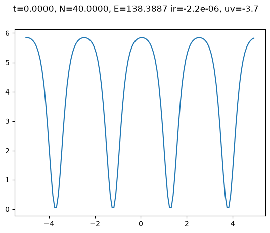
from gpe.minimize import MinimizeStateFixedPhase
 
s = State(Nx=128)
s.set_psi(2)
Nx = s.shape[0]
N = 2
phase = np.sign(np.exp(2j*np.pi * N * np.arange(Nx) / Nx).real)
s = MinimizeStateFixedPhase(s, phase).minimize()
s.plot()
 

[<Axes: >]

../_images/b5a38cd5e8d2eca9d4696b34fb9c0c42e67141a9401005153604505e593224b3.png

{code-cell} ipython3
%%time
Nx = 256*16*16
s = State(eps=0.1, g=-1. Nxyz=(Nx,), Lxyz=(128*Nx/2**16,))
T = 3.5
Nt = 100
dT = T/Nt
dt = 0.2*s.t_scale
steps = int(np.ceil(dT/dt))
dt = dT/steps
ev = EvolverABM(s, dt=dt)
ss = [s]
fig, ax = plt.subplots()
for n in FPS(Nt, fig=fig, embed=True, display=True):
    ev.evolve(steps)
    ss.append(ev.get_y())
    ax.cla()
    ev.y.plot(axs=[ax])

{code-cell} ipython3
k4s = []
ts = []
for s in ss:
    n = s.get_density()
    k4 = s.basis.Lxyz[0] * s.integrate(n**2) / s.integrate(n)**2
    k4s.append(k4)
    ts.append(s.t)

fig, ax = plt.subplots()
ax.plot(ts, k4s)
ax.set(xlabel="$t$", ylabel="$k_4(t)$");

{code-cell} ipython3