General Theory - Sum Rules
A general formulation of linear response is discussed in [Pitaevskii and Stringari, 2003] and we
summarize their results here. The idea is to start consider two linear operators: one
\(\op{G}\) that creates the excitation, and another \(\op{F}\) that we measure to detect the
excitation. The system evolves with a hermitian Hamiltonian
\[\begin{gather*}
\op{H}_{\lambda}(t) = \op{H} + \lambda e^{0^+ t}\op{H}_{\text{pert}}(t), \qquad
\op{H}_{\text{pert}} = -(\op{G}e^{\omega t/\I} + \text{h.c.}).
\end{gather*}\]
We then consider the linear response in terms of the expectation-value of the
operator \(\op{F}\):
\[\begin{gather*}
\delta\braket{\op{F}} = \lambda e^{0^+ t}(
\chi_{F, G}(\omega)e^{\omega t /\I} + \text{h.c})
= \lambda e^{0^+ t}(
\chi_{F, G}(\omega)e^{\omega t /\I} +
\underbrace{\chi_{F, G}(-\omega)}_{\chi_{F, G}^*(\omega)}e^{-\omega t /\I}).
\end{gather*}\]
If we consider a time-independent Hamiltonian \(\op{H}\) and start with a system in
thermal equilibrium at \(t=-\infty\) with temperature \(T\), we
obtain
\[\begin{gather*}
\chi_{F,G}(\omega) =
-\frac{1}{Q\hbar}\sum_{mn}
e^{-\beta E_m}
\Biggl(
\frac{\braket{m|\op{F}|n}\braket{n|\op{G}|m}}
{\omega_+ - \omega_{nm}}
-
\frac{\braket{m|\op{G}|n}\braket{n|\op{F}|m}}
{\omega_+ + \omega_{nm}}
\Biggr). \tag{7.3}
\end{gather*}\]
Do It! Derive this.
Hint: Consider the density matrix.
Recall that a thermal ensemble can be described in terms of the energy eigenstates
\(\ket{n}\) by a density matrix
\[\begin{gather*}
\op{R} = \sum_{n} \ket{n}e^{-\beta E_{n}}\bra{n}, \qquad
\op{H}\ket{n} = \ket{n}E_n, \qquad
\beta = \frac{1}{k_B T},\\
\braket{\op{F}} = \Tr \op{R}\op{F} = \sum_{n}\frac{e^{-\beta
E_n}}{Q}\braket{n|\op{F}|n},\qquad
Q = \sum_{n} e^{-\beta E_n}.
\end{gather*}\]
The time-evolution of this state is
\[\begin{gather*}
\op{R}(t) = \sum_{n} \ket{n(t)}e^{-\beta E_{n}}\bra{n(t)}, \\
\I\hbar\partial_t\ket{n(t)} = \op{H}_{\lambda}(t)\ket{n(t)}, \qquad
\ket{n(-\infty)} = \ket{n}.
\end{gather*}\]
Solution
I find it easiest to work with the operator representations of these equations:
\[\begin{gather*}
\I \hbar \partial_{t}\op{R}(t) = [\op{H}_{\lambda}(t), \op{R}(t)], \qquad
\op{R}(-\infty) = e^{-\beta \op{H}}.
\end{gather*}\]
At linear order, there will be no mixing of frequencies, thus, since our perturbation
contains only \(e^{\pm \omega t/\I}\), the response will have the same form. We thus
include this from the start (but one can check this more generally if
desired). Expanding to linear order, we have
\[\begin{gather*}
\op{R}(t) = \op{R}
+ \lambda \underbrace{(\delta\op{R}_{+}e^{\omega t/\I} + \text{h.c.})}_{\delta \op{R}(t)}
+ O(\lambda^2),\\
\I\hbar \partial_t \delta \op{R}(t)
=
[\op{H}, \delta\op{R}(t)] + [\op{H}_{\text{pert}}(t), \op{R}] + O(\lambda),\\
\hbar \omega_+ \delta \op{R}_{+} = [\op{H}, \delta\op{R}_{+}] - [\op{G}, \op{R}]\\
-\hbar \omega_- \delta \op{R}_{+}^\dagger
= [\op{H}, \delta\op{R}_{+}^\dagger] - [\op{G}^\dagger, \op{R}]
\end{gather*}\]
where we have included the convergence factors in
\[\begin{gather*}
\omega_{\pm} = \omega \pm \I 0^+.
\end{gather*}\]
Now we can compute the response
\[\begin{gather*}
Q\delta \braket{\op{F}} = \lambda \Bigl(
e^{\omega_+ t/\I}\Tr(\delta\op{R}_+\op{F})
+ e^{-\omega_- t/\I}\Tr(\delta\op{R}_+^\dagger\op{F})
\Bigr)
\end{gather*}\]
The desired result comes from inserting a complete set of states
\[\begin{multline*}
Q\delta \braket{\op{F}} = \lambda \Bigl(
e^{\omega_+ t/\I}\sum_{mn}\braket{n|\delta\op{R}_+|m}\braket{m|\op{F}|n} \\
+ e^{-\omega_- t/\I}
\sum_{mn}\braket{n|\delta\op{R}_+^\dagger|m}\braket{m|\op{F}|n}
\Bigr).
\end{multline*}\]
Taking the matrix elements of the linear response equation, and using the fact that
\(\op{H}\ket{n} = \ket{n}E_n\) and \(\op{R}\ket{n} = \ket{n}e^{-\beta E_n}\) are diagonal, we
obtain
\[\begin{gather*}
\hbar \omega_+ \braket{n|\delta\op{R}_+|m} = \Bigl(
(E_n-E_m)\braket{n|\delta\op{R}_{+}|m}
+
(e^{-\beta E_n}-e^{-\beta E_m})\braket{n|\op{G}|m}
\Bigr),\\
\braket{n|\delta\op{R}_+|m}
= \frac{e^{-\beta E_n}-e^{-\beta E_m}}{\hbar \omega_+ - \underbrace{(E_n-E_m)}_{\hbar\omega_{nm}}}
\braket{n|\op{G}|m}.
\end{gather*}\]
Assembling everything, we have
\[\begin{gather*}
\delta \braket{\op{F}} = \frac{\lambda}{\hbar Q} \Biggl(
e^{\omega_+ t/\I}
\sum_{mn}\frac{(e^{-\beta E_n} - e^{-\beta
E_m})\braket{n|\op{G}|m}\braket{m|\op{F}|n}}{\omega_+ - \omega_{nm}} + \text{h.c.}\Biggr),
\end{gather*}\]
from which we can read off the stated result, after rearranging some indices.
The sum-rule associated with an operator \(\op{F}\) has the form (see [Wang, 1999])
\[\begin{gather*}
\sum_{m}(E_{m} - E_{0})\abs{\braket{m|\op{F}|0}}^2 =
\braket{0|[\op{F},\op{H}]\op{F}^\dagger|0}.
\end{gather*}\]
These are useful if the final commutators have simple forms.
Do it! Derive this.
Simply insert a complete set of energy eigenstates:
\[\begin{align*}
\braket{0|[\op{F},\op{H}]\op{F}^\dagger|0} &=
\sum_{m}\braket{0|[\op{F},\op{H}]|m}\braket{m|\op{F}^\dagger|0}\\
&= \sum_{m}(\braket{0|\op{F}\op{H}|m}-\braket{0|\op{H}\op{F}|m})\braket{m|\op{F}^\dagger|0}\\
&= \sum_{m}(\braket{0|\op{F}|m}E_{m} - E_0\braket{0|\op{F}|m})\braket{m|\op{F}^\dagger|0}\\
&= \sum_{m}(E_{m} - E_{0})\braket{0|\op{F}|m}\braket{m|\op{F}^\dagger|0}\\
= \sum_{m}(E_{m} - E_{0})\abs{\braket{m|\op{F}|0}}^2.
\end{align*}\]
Here we consider the fluctuations about a stationary state \(\psi_0\) of GPE-like
theories to linear order – sometimes called Bogoliubov theory.
Bogoliubov Theory
We assume that the equations of motion (EoM) arise from a principle of
stationary action:
\[\begin{gather*}
S[\psi] = \int \left(\int \I\hbar \psi^\dagger\dot{\psi} \d{x} - E[\psi]\right)\d{t},\\
\I\hbar \dot{\psi} = \op{H}[\psi]\psi = \frac{\delta E[\psi]}{\delta \psi^\dagger}.
\end{gather*}\]
For standard GPE-like theories, we have
\[\begin{gather*}
E[\psi] = \int \d{x}\; \left(
\psi^{\dagger}K(\op{p})\psi + \mathcal{E}(n)
\right), \qquad
n = \abs{\psi}^2,\\
\I\hbar \dot{\psi} = \Bigl(K(\op{p}) + \mathcal{E}'(n)\Bigr)\psi,
\end{gather*}\]
where \(\mathcal{E}(n)\) is the equation of state and \(K(\op{p})\) is the single-particle
dispersion relation (kinetic energy). More generally, we might have
an external potential, chemical potential, etc. We roll all of these into
\(\mathcal{E}(n)\) for this discussion and keep this general. Thus, for the standard GPE
we would have
\[\begin{gather*}
K_{GPE}(\op{p}) = \frac{\op{p}^2}{2m} = \frac{-\hbar^2\nabla^2}{2m},\\
\mathcal{E}_{GPE}(n) = g\frac{n^2}{2} + V(x, t)n,\\
\I\hbar \dot{\psi} = \Biggl(
\underbrace{\frac{-\hbar^2\nabla^2}{2m}}_{K(\op{p})}
+ \underbrace{gn + V(x, t)}_{\mathcal{E}'_{GPE}(n)}
\Biggr)\psi.
\end{gather*}\]
We now replace the spatial dependence with the usual Hilbert-space structure, and express
the equations of motion in terms of kets:
\[\begin{gather*}
\I\hbar \dot{\ket{\psi}} = \op{H}[\psi]\ket{\psi}, \qquad
\psi(x) = \braket{x|\psi}.
\end{gather*}\]
The idea of Bogoliubov theory is to consider fluctuations about a stationary state
\(\ket{\psi_0}\):
\[\begin{gather*}
\overbrace{\op{H}[\psi_0]}^{\op{H}_0}\ket{\psi_0} = \ket{\psi_0}\mu,\qquad
\ket{\psi} = e^{\mu t/\I\hbar}\Bigl(
\ket{\psi_0}
+ \overbrace{\underbrace{\ket{u_+}}_{\ket{u}}e^{\omega t/\I}
+ \underbrace{\ket{u_-}}_{-\ket{v^*}}e^{-\omega^* t/\I}}^{\ket{u}}
\Bigr),
\end{gather*}\]
finding \(\ket{u_{\pm}}\) that satisfy the equations of motion to linear order. The
presence of the non-linear term \(n(x) = \braket{x|\psi}\braket{\psi|x}\) mixes the
positive and negative frequency components. Specifically
\[\begin{alignat*}{2}
n(x) &= n_0(x) &&+ \overbrace{u(x)\psi_0^*(x) + \text{h.c.}}^{\delta n(x)} \\
&= n_0(x) &&
+ u_{+}(x)e^{\omega t/\I}\psi_0^*(x)
+ u_{-}(x)e^{-\omega^* t/\I}\psi_0^*(x)\\
&&& + u_{+}^*(x)e^{-\omega^* t/\I}\psi_0(x)
+ u_{-}^*(x)e^{\omega t/\I}\psi_0(x),\\
&= n_0(x)
&&+ e^{\omega t/\I}\Bigl(u_+(x)\psi_0^*(x) + u_-^*(x)\psi_0(x)\Bigr)\\
&&&+ e^{-\omega^* t/\I}\Bigl(u_-(x)\psi_0^*(x) + u_+^*(x)\psi_0(x)\Bigr)
+ O(u^2).
\end{alignat*}\]
Expanding the Hamiltonian to linear order, we thus have
\[\begin{gather*}
\op{H}[\psi] = \op{H}_0
+ \mathcal{E}''(n_0)\overbrace{(u\psi_0^* + u^*\psi_0)(\op{x})}^{
u(\op{x})\psi_0^*(\op{x}) + u^*(\op{x})\psi_0(\op{x})}
+ O(u)^2.
\end{gather*}\]
Finally, expanding the equation of motion and multiplying through by \(e^{-\mu t
/\I\hbar}\), we have
\[\begin{gather*}
\mu \overbrace{\ket{\psi}e^{-\mu t /\I\hbar}}
^{\ket{\psi_0} + \ket{u}} + \I\hbar\dot{\ket{u}}
= \overbrace{\op{H}_0\ket{\psi_0}}^{\ket{\psi_0}\mu} + \op{H}_0\ket{u}
+ \mathcal{E}''(n_0)(u\psi_0^* + u^*\psi_0)(\op{x})\ket{\psi_0} + O(u^2),\\
\ket{u}\mu + \I\hbar\dot{\ket{u}}
= \op{H}_0\ket{u}
+ \mathcal{E}''(n_0)(u\psi_0^* + u^*\psi_0)(\op{x})\ket{\psi_0} + O(u^2).
\end{gather*}\]
We now expand \(\ket{u} = \ket{u_+}e^{\omega t/\I} +
\ket{u_-}e^{-\omega^* t/\I}\), and collect the positive and negative frequency
terms, demanding that both vanish independently.
\[\begin{gather*}
u_+\mu + \hbar\omega u_+
= \braket{x|\op{H}_0|u_+}
+ \mathcal{E}''(n_0)(u_+\psi_0^* + u_{-}^*\psi_0)\psi_0,\\
u_-\mu - \hbar\omega^* u_-
= \braket{x|\op{H}_0|u_-}
+ \mathcal{E}''(n_0)(u_-\psi_0^* + u_{+}^*\psi_0)\psi_0.
\end{gather*}\]
These can be packaged as a generalized eigenvalue equation after conjugating the second equation
\[\begin{gather*}
\begin{pmatrix}
\op{H}_0 - \mu + n_0\mathcal{E}''(n_0) & \psi_0^2\mathcal{E}''(n_0)\\
(\psi^*_0)^2\mathcal{E}''(n_0) & \op{H}_0^* - \mu + n_0\mathcal{E}''(n_0)
\end{pmatrix}
\begin{pmatrix}
u_+\\
u_-^*
\end{pmatrix}
=
\hbar\omega
\begin{pmatrix}
1\\
& -1
\end{pmatrix}
\begin{pmatrix}
u_+\\
u_-^*
\end{pmatrix}.
\end{gather*}\]
On Conjugate Pairs of Eigenvalues: \(\omega_n\), \(-\omega_n^*\).
This is a generalized eigenvalue problem of the form \(\mat{A}\ket{n} =
\mat{B}\ket{n}\omega_{n}\) with Hermitian matrices \(\mat{A} = \mat{A}^\dagger\) and
\(\mat{B} = \mat{B}^\dagger\). Numerically this generalized eigenvalue problem is easy to
work with if \(\mat{B}\) is positive definite – i.e. has positive eigenvalues (see
e.g. scipy.linalg.eigh()). In this case we can use its diagonalization to write
\[\begin{gather*}
\mat{B} = \mat{U}^\dagger\mat{D}\mat{U}
=\mat{U}^\dagger\sqrt{\mat{D}}\mat{U}
\underbrace{\mat{U}^\dagger\sqrt{\mat{D}}\mat{U}}_{\mat{b}}
= \mat{b}^\dagger\mat{b},
\end{gather*}\]
where \(\mat{b}\) is invertable since \(\mat{D}\) is diagonal with positive entries.
Then we have a hermitian problem \(\tilde{\mat{A}}\tilde{\ket{n}} = \tilde{\ket{n}}\omega_n\) with
\[\begin{gather*}
\mat{A}\mat{b}^{-1}\mat{b}\ket{n} = \mat{b}^\dagger\mat{b}\ket{n}\omega_{n}\\
\underbrace{(\mat{b}^{-1})^\dagger\mat{A}\mat{b}^{-1}}_{\tilde{\mat{A}}}
\underbrace{\mat{b}\ket{n}}_{\tilde{\ket{n}}}
= \underbrace{\mat{b}\ket{n}}_{\tilde{\ket{n}}}\omega_{n}.
\end{gather*}\]
I.e., we can transform the problem into a standard Hermitian eigenvalue problem.
In our case, unfortunately, \(\mat{B}\) is not positive definite, making the problem
somewhat challenging. There are some nice properties of our system, however (see
e.g. [Wu and Niu, 2003]). Specifically, we can write the as \(\mat{B} = \mat{Z}\) where
\(\mat{Z} = \mat{\sigma}_{z}\otimes \mat{1}\). These following from the property that
\[\begin{gather*}
\mat{X}\mat{A}\mat{X} = \mat{A}^*, \qquad \mat{X}\mat{B}\mat{X} = -\mat{B}^*
\end{gather*}\]
where \(\mat{X} = \mat{\sigma}_{x}\otimes \mat{1}\). Hence, if \(\ket{n}\) is an eigenvector
with eigenvalue \(\omega_{n}\), then \(\mat{X}\ket{n}^*\) is an eigenvector with eigenvalue
\(-\omega_{n}^*\):
\[\begin{gather*}
\mat{A}\ket{n} = \mat{B}\ket{n}\omega_n\\
\mat{X}\mat{A}\mat{X}\mat{X}\ket{n} = \mat{X}\mat{B}\mat{X}\mat{X}\ket{n}\omega_n\\
\mat{A}^*\mat{X}\ket{n} = -\mat{B}^*\mat{X}\ket{n}\omega_n\\
\mat{A}\mat{X}\ket{n}^* = \mat{B}\mat{X}\ket{n}^*(-\omega_n^*).
\end{gather*}\]
Thus, all eigenvalues with non-zero real parts appear in conjugate pairs \(\omega_n\) and
\(-\omega_n^*\). Purely imaginary eigenvalues may in principle be isolated, but will have
eigenvectors which satisfy \(\mat{X}\ket{n}^* = \ket{n}\).
In many cases – for example, if the dispersion relationship is quadratic \(K(p) =
p^2/2m\), the matrix \(\mat{A}=\mat{A}^*\) is self-conjugate and \(\mat{B}^* = -\mat{B}\).
(This may not be the case with more complicated dispersions that break parity for
example.) In these cases, we can further simplify the equations. Introduce the
following projectors:
\[\begin{gather*}
\mat{P}_{\pm} = \frac{\mat{1} \pm \mat{Z}}{2}, \qquad
\mat{X}\mat{P}_{\pm}\mat{X} = \mat{P}_{\pm}.\\
\ket{n} = \frac{\mat{X} + \mat{Z}}{\sqrt{2}}\ket{\tilde{n}},\\
\mat{A}\ket{n} = \frac{\mat{A}\mat{X} + \mat{A}\mat{Z}}{\sqrt{2}}\ket{\tilde{n}},\\
\end{gather*}\]
\[\begin{gather*}
\mat{P}_{+}\mat{A}\mat{P}_{+}\mat{P}_{-}\mat{A}\mat{P}_{-}\ket{\tilde{n}} =\ket{\tilde{n}}\omega_n
\end{gather*}\]
HAH = P()P + M()M
HAH = (X+Z)A(X+Z)/2
= (XAX + ZAZ + XAZ + ZAX)/2
= (4A + ZAZ + AXZ + ZXA)/2
On the \(\psi_0^2\) off-diagonals: \(\tilde{K}(\op{p})\).
The factor of \(\psi_0^2\) and conjugate in the off-diagonals is a nuisance, since the
corresponding factor of \(n_0\) appears on the diagonals. In many cases, one can take the
stationary state \(\psi_0 = \psi_0^*\) to be real, in which case \(\psi_0^2 = n_0\), but
there are examples where this cannot be done (states with twisted boundary conditions
for example, as discussed below).
In these cases, the terms differ by a phase \(\psi_0^2 = e^{2\I\phi}n_0\) which can be
absorbed in a redefinition of \(u_{-} \rightarrow e^{2\I\phi} u_{-}^*\). If
the phase is spatially dependent, however, then this operation will generally not commute with
the kinetic energy but can be convenient. The argument goes like this (and shows a more
streamlined calculation):
First include the chemical potential in \(\op{H}_0 = \op{H}[\psi_0] - \mu\op{1}\) so that
\(\op{H}_0\psi_0 = 0\), and consider the state
\[\begin{gather*}
\op{H}_0\psi_0 = 0, \qquad
\psi = \psi_0(1 + \epsilon) = \psi_0 + \psi_0\epsilon, \qquad
\epsilon = \epsilon_+ e^{\omega t/\I} + \epsilon_- e^{-\omega t/\I}.
\end{gather*}\]
The expansion of the density now contains only \(n_0\): no factors of \(\psi_0\) or
\(\psi_0^*\) remain:
\[\begin{gather*}
n = n_0(1 + \epsilon + \epsilon^*) + O(\epsilon^2).
\end{gather*}\]
Inserting this into the EoM and keeping terms of order \(\epsilon\), we have
\[\begin{gather*}
\I \hbar \psi_0\dot{\epsilon} =
\op{H}_0(\psi_0\epsilon) + \mathcal{E}''(n_0)n_0(\epsilon + \epsilon^*)\psi_0.
\end{gather*}\]
The last term – from the expansion of \(n\) – contains both \(\epsilon\) and
\(\epsilon^*\). This is a consequence of the non-linear nature of the GPE-like equation
and gives rise to a coupled set of equations for the linear response. In this case,
there are no terms like \(\psi_0^2\) as in the original derivation. The factored
perturbation simply gives \(n_0\) factors with the complication that \(\op{H}_0\) now acts
on the product \(\psi_0\epsilon\). To proceed, we must define a new operator
\(\op{\tilde{H}}_0\) that satisfies
\[\begin{gather*}
\op{H}_0(\psi_0 \epsilon) = \psi_0\op{\tilde{H}_0}(\epsilon).
\end{gather*}\]
Only the kinetic energy is a problem, so we really just need to an operator
\(\tilde{K}(\op{p})\) such that
\[\begin{gather*}
K(\op{p})(\psi_0\epsilon) = \psi_0\tilde{K}(\op{p})\epsilon.
\end{gather*}\]
Then we can express these equations as
\[\begin{gather*}
\begin{pmatrix}
\op{\tilde{H}} + n_0\mathcal{E}'' - \hbar \omega & n_0\mathcal{E}''\\
n_0\mathcal{E}'' & \op{\tilde{H}}^* + n_0\mathcal{E}'' + \hbar \omega^*
\end{pmatrix}
\begin{pmatrix}
\epsilon_+\\
\epsilon_-^*
\end{pmatrix}
=
\vect{0},\\
\op{\tilde{H}} = \tilde{K}(\op{p}) + \mathcal{E}'(n_0) + V(x, t) - \mu.
\end{gather*}\]
This modified approach will be useful when we can explicitly form \(\tilde{K}(\op{p})\).
Consider how this works for various powers of \(p\) as a consequence of the General Leibniz rule
\[\begin{align*}
\op{p}(\psi_0\epsilon) &= (\op{p}\psi_0) \epsilon + \psi_0(\op{p}\epsilon)\\
\op{p}^2(\psi_0\epsilon) &=
(\op{p}^2\psi_0) \epsilon + 2(\op{p}\psi_0)(\op{p}\epsilon) + \psi_0(\op{p}^2\epsilon),\\
\op{p}^n(\psi_0\epsilon) &= \sum_{m=0}^{n}\binom{n}{m}(\op{p}^{m}\psi_0)(\op{p}^{n-m} \epsilon).
\end{align*}\]
For the usual quadratic dispersion \(K(\op{p}) = \op{p^2}/2m\) and expanding about a state
\(\psi_0\) with momentum \(p_0\), we have
\[\begin{align*}
\tilde{K}(\op{p}) = \frac{(p_0+\vect{p})^2}{2m}
= \frac{p_0^2}{2m} + \frac{p_0\op{p}}{m} + \frac{\op{p}^2}{2m}
= E_0 + v_0\op{p} + \frac{\op{p}^2}{2m},\\
\tilde{K}^*(\op{p}) = \frac{(p_0-\vect{p})^2}{2m}
= \frac{p_0^2}{2m} - \frac{p_0\op{p}}{m} + \frac{\op{p}^2}{2m}
= E_0 - v_0\op{p} + \frac{\op{p}^2}{2m}.
\end{align*}\]
Note that \(\op{p}^* = -\op{p}\). This is exactly the transformation required to restore
Galilean invariance. I.e., the normal modes about the state \(\psi_0\) with momentum
\(p_0\) (and velocity \(v_0=p_0/m\)) should be the same as the normal modes in a co-moving
frame where \(\psi_0\) has zero momentum. More on this below.
Solving the Bogoliubov Equations.
For this discussion, we will consider the following form of the Bogoliubov equations:
\[\begin{gather*}
\begin{pmatrix}
\mat{A} & \mat{B}\\
\mat{B} & \mat{A}^*
\end{pmatrix}
\begin{pmatrix}
u_{+}\\
u_{-}^*
\end{pmatrix}
=
\mat{z}
\begin{pmatrix}
u_{+}\\
u_{-}^*
\end{pmatrix}
\omega, \qquad
\mat{z} = \begin{pmatrix}
\mat{1}\\
& -\mat{1}
\end{pmatrix}.
\end{gather*}\]
This can be written as a non-hermitian eigenvalue problem by letting \(u=u_{+}\) and \(v =
-u_{-}^*\), recovering the form of the Bogoliubov-de Gennes (BdG) equations seen in the
Hartree-Fock-Bogoliubov (HFB) theory of superconductivity:
\[\begin{gather*}
\begin{pmatrix}
\mat{A} & -\mat{B}\\
\mat{B} & -\mat{A}^*
\end{pmatrix}
\begin{pmatrix}
u\\
v
\end{pmatrix}
=
\begin{pmatrix}
u\\
v
\end{pmatrix}
\omega.
\end{gather*}\]
To make further progress, consider
\[\begin{gather*}
\begin{pmatrix}
\alpha\\
\beta
\end{pmatrix}
=
\frac{1}{\sqrt{2}}
\begin{pmatrix}
\mat{1} & \mat{1}\\
\mat{1} & -\mat{1}
\end{pmatrix}
\begin{pmatrix}
u\\
v
\end{pmatrix},\\
\frac{1}{2}
\begin{pmatrix}
\mat{1} & \mat{1}\\
\mat{1} & -\mat{1}
\end{pmatrix}
\begin{pmatrix}
\mat{A} & -\mat{B}\\
\mat{B} & -\mat{A}^*
\end{pmatrix}
\begin{pmatrix}
\mat{1} & \mat{1}\\
\mat{1} & -\mat{1}
\end{pmatrix}
\begin{pmatrix}
\alpha\\
\beta
\end{pmatrix}
=
\begin{pmatrix}
\alpha\\
\beta
\end{pmatrix}
\omega,\\
\frac{1}{2}
\begin{pmatrix}
\mat{A}-\mat{A}^* & \mat{A} + \mat{A}^* + 2\mat{B}\\
\mat{A} + \mat{A}^* - 2\mat{B} & \mat{A} - \mat{A}^*
\end{pmatrix}
\begin{pmatrix}
\alpha\\
\beta
\end{pmatrix}
=
\begin{pmatrix}
\alpha\\
\beta
\end{pmatrix}
\omega.
\end{gather*}\]
\[\begin{gather*}
\begin{pmatrix}
\mat{A} & \I\mat{B}\\
\I\mat{B} & -\mat{A}^*
\end{pmatrix}
\begin{pmatrix}
u_{+}\\
\I u_{-}^*
\end{pmatrix}
=
\begin{pmatrix}
u_{+}\\
\I u_{-}^*
\end{pmatrix}
\omega,
\end{gather*}\]
array([[ 1.11200000e+01-2.23711432e-17j, -2.42933074e-16+1.00000000e+00j],
       [-4.71276680e-16+1.00000000e+00j,  1.08800000e+01-2.23711432e-17j]])
Homogeneous Matter
To see how this works, consider homogeneous matter where \(\psi_0\) has momentum \(\hbar k_0\).
Translation invariance implies that we can use plane-waves \(u_{\pm} = \sqrt{n_0}\epsilon_{\pm}e^{\I
(k_0 \pm k) x}\).
\[\begin{gather*}
\psi = \sqrt{n_0}e^{\I (k_0 x - \mu t/\hbar)}\Bigl(
1 + \epsilon_+ e^{\I(kx - \omega t)} + \epsilon_- e^{-\I(kx - \omega t)}
\Bigr),\\
= e^{\mu t/\hbar \I}\Bigl(
\sqrt{n_0}e^{\I k_0 x}
+ \sqrt{n_0}\epsilon_+ e^{\I\bigl((k+k_0)x - \omega t\bigr)}
+ \sqrt{n_0}\epsilon_- e^{-\I\bigl((k-k_0)x - \omega t\bigr)}
\Bigr).
\end{gather*}\]
In this case \(\op{H}\) and \(\op{H}^*\) can be treated as a numbers
\[\begin{gather*}
H = \frac{\hbar^2(k_0 + k)^2}{2m} + \mathcal{E}'(n_0) - \mu, \qquad
H^* = \frac{\hbar^2(k_0 - k)^2}{2m} + \mathcal{E}'(n_0) - \mu.
\end{gather*}\]
We start by expanding about the ground state with \(k_0=0\) so that \(H = H^*\). Taking the
determinant, we have
\[\begin{gather*}
H^2 + 2Hn_0\mathcal{E}''(n_0) - H \hbar (\omega - \omega^*) - \hbar^2\abs{\omega}^2 = 0.
\end{gather*}\]
If \(\omega = \omega^*\), then we find the usual phonon dispersion relation:
\[\begin{gather*}
\hbar\omega(k) = \pm\sqrt{H(H + 2n_0\mathcal{E}'')}
= \pm\sqrt{H(H + 2mc^2)},\qquad
c = \sqrt{\frac{n_0\mathcal{E}''(n_0)}{m}},
\end{gather*}\]
where (as we shall see shortly) \(c\) is the long wavelength speed of sound, expressed in
terms of the compressibility \(\mathcal{E}''(n_0)\).
The chemical potential \(\mu\) cancels the constant pieces so that \(\op{H}\psi_0 = 0\) and:
\[\begin{gather*}
H = \frac{\hbar^2 k^2}{2m}.
\end{gather*}\]
Phonon Dispersion
This gives the familiar dispersion of phonons about the ground state \(p_0 = 0\):
\[\begin{align*}
\omega(k) &= \pm ck
\sqrt{1 + \frac{\hbar^2k^2}{4m^2c^2}}, &
c &= \sqrt{\frac{n_0\mathcal{E}''(n_0)}{m}},\\
E(p) = \hbar\omega &= \pm cp
\sqrt{1 + \frac{p^2}{2m} \frac{1}{2mc^2}}.
\end{align*}\]
This is linear in the long wavelength limit \(k \rightarrow 0\) with the advertised speed
of sound \(c\). Note that when expressed in terms of the energy and momentum, this is a
classical result without any explicit factors of \(\hbar\).
More generally, expanding about state \(\psi_0\) with momentum \(p_0\),
\[\begin{gather*}
H = \overbrace{\frac{\hbar^2k^2}{2m}}^{H_0} + v_0k = \frac{\hbar^2(k+k_0)^2}{2m} - E_0,\\
H^* = \frac{\hbar^2k^2}{2m} - v_0k = \frac{\hbar^2(k-k_0)^2}{2m} - E_0,\\
\begin{vmatrix}
H_0 - \hbar(\omega - v_0k) + n_0\mathcal{E}''(n_0) & n_0\mathcal{E}''(n_0)\\
n_0\mathcal{E}''(n_0) & H_0 + \hbar(\omega - v_0k)^* + n_0\mathcal{E}''(n_0)
\end{vmatrix} = 0
\end{gather*}\]
where \(v_0 = p_0/m\) and \(E_0 = mv_0^2/2\). Taking the determinant, we have the slightly
more cumbersome
\[\begin{gather*}
H_0^2 + 2H_0n_0\mathcal{E}''(n_0) - H_0 \hbar (\omega - \omega^*)
- \hbar^2\abs{(\omega-v_0k)}^2 = 0.
\end{gather*}\]
And if \(\omega = \omega^*\), we find the boosted phonon dispersion:
\[\begin{gather*}
\hbar\omega(k) - v_0k = \pm\sqrt{H_0(H_0 + 2n_0\mathcal{E}'')}.
\end{gather*}\]
Counterflow Instability
As an application, consider a miscible (\(g_{ab}^2 < g_{aa}g_{bb}\)) two-component
superfluid. The homogeneous system becomes unstable if the two components flow past
each other at a sufficiently large relative velocity \(\abs{v_a - v_b} > v_c\) – a
counterflow instability. Here we use the Bogoliubov theory to see this instability.
The Hamiltonian is derived by varying the following self-energy:
\[\begin{gather*}
\mathcal{E}(n_a, n_b) = \cdots + \frac{1}{2}\vect{n}^\dagger\mat{g}\vect{n},
\qquad
\mat{g} = \begin{pmatrix}
g_{aa} & g_{ab}\\
g_{ab} & g_{bb}
\end{pmatrix},
\qquad
\vect{n} = \begin{pmatrix}
n_a\\
n_b
\end{pmatrix}.
\end{gather*}\]
We consider perturbing the following state
\[\begin{gather*}
\ket{\psi_0} = \begin{pmatrix}
\sqrt{n_a}e^{\I q x + \mu_a t/\I\hbar}\\
\sqrt{n_b}e^{-\I q x + \mu_b t/\I\hbar}
\end{pmatrix}, \qquad
\mu_a = \frac{\hbar^2q^2}{2m} + g_{aa}n_a + g_{ab}n_b, \qquad
\mu_b = \frac{\hbar^2q^2}{2m} + g_{ab}n_a + g_{bb}n_b.
\end{gather*}\]
To this we add a perturbation
\[\begin{gather*}
\ket{u} = \begin{pmatrix}
u_a\sqrt{n_a}e^{\I q x + \mu_a t/\I\hbar}\\
u_b\sqrt{n_b}e^{-\I q x + \mu_b t/\I\hbar}
\end{pmatrix}e^{\I (kx - \omega t)}
-
\begin{pmatrix}
v_a^*\sqrt{n_a}e^{\I q x + \mu_a t/\I\hbar}\\
v_b^*\sqrt{n_b}e^{-\I q x + \mu_b t/\I\hbar}
\end{pmatrix}e^{-\I (kx - \omega t)},\\
\delta \vect{n} = \begin{pmatrix}
n_a(u_a - v_a)\\
n_b(u_b - v_b)
\end{pmatrix}
e^{\I(kx-\omega t)}
+
\begin{pmatrix}
n_a(u_a^* - v_a^*)\\
n_b(u_b^* - v_b^*)
\end{pmatrix}
e^{-\I(kx-\omega t)} + \cdots
\end{gather*}\]
These give rise to the following Bogoliubov equations
\[\begin{gather*}
\begin{pmatrix}
\overbrace{K(q\mat{z} + k\mat{1}) - K(q\mat{z})}
^{\frac{(\hbar k)^2}{2m}\mat{1} + \hbar k v \mat{z}}
+ \mat{gn} - \hbar\omega \mat{1} & \mat{gn}\\
\mat{gn} & \underbrace{K(q\mat{z} - k\mat{1}) - K(q\mat{z})}
_{\frac{(\hbar k)^2}{2m}\mat{1} - \hbar k v \mat{z}}
+ \mat{gn} + \hbar\omega \mat{1} \\
\end{pmatrix}
\begin{pmatrix}
u_{a}\\
u_{b}\\
-v_{a}\\
-v_{b}
\end{pmatrix}
= 0,
\end{gather*}\]
where \(K(k) = \hbar^2k^2/2m\), and
\[\begin{gather*}
\mat{gn} =
\begin{pmatrix}
g_{aa}n_{a} & g_{ab}n_b \\
g_{ab}n_{a} & g_{bb}n_b
\end{pmatrix},\\
K(q\mat{z} \pm k\mat{1}) - K(q\mat{z})
= \frac{\hbar^2}{2m}k\Bigl(k\mat{1} \pm 2 q\mat{z}\Bigr)
= \frac{(\hbar k)^2}{2m}\mat{1} \pm \hbar k v \mat{z},\\
v = \frac{\hbar q}{m} = v_a = -v_b.
\end{gather*}\]
The structure of the equations is then
\[\begin{gather*}
\mat{M} = \begin{pmatrix}
\frac{\hbar^2 k^2}{2m}\mat{1} + \hbar k v \mat{z}
+ \mat{gn} & -\mat{gn}\\
\mat{gn} & -\frac{\hbar^2 k^2}{2m}\mat{1} + \hbar k v \mat{z}
- \mat{gn}\\
\end{pmatrix},\\
(\mat{M} - \hbar \omega \mat{1})
\begin{pmatrix}
u_{a}\\
u_{b}\\
v_{a}\\
v_{b}
\end{pmatrix}
= 0.
\end{gather*}\]
Nonlinear Terms: \(\mat{gn}\).
Consider the equation of \(\psi_a\). It contains the non-linear term
\[\begin{gather*}
\I\hbar \dot{\psi}_a = \cdots + (g_{aa}n_a + g_{ab}n_b)\psi_a.
\end{gather*}\]
Expanding this will give three contributions – two from expanding the densities, and
one from expanding \(\psi_a\) itself. The piece obtained by expanding \(\psi_a\) will
cancel will the chemical potential \(\mu_a\), so we will only have the other two terms.
Considering the equation with \(e^{-\I\omega t\) for \(u_a\), we will have
which have the form
\[\begin{gather*}
\hbar \omega \sqrt{n_a}u_a = \cdots
+ g_{aa}n_a (u_a - v_a)\sqrt{n_a}
+ g_{ab}n_b(u_b - v_b)\sqrt{n_a}.
\end{gather*}\]
\[\begin{gather*}
\begin{pmatrix}
g_{aa}n_a & g_{ab}n_b & g_{aa}n_a & g_{ab}n_b\\
g_{aa}n_a & g_{ab}n_b & g_{aa}n_a & g_{ab}n_b\\
\vdots
\end{pmatrix}
\end{gather*}\]
Determinant of \(\mat{M}\) (incomplete).
To compute the determinant of \(\mat{M}\), we first write the tensor structure in terms of
the 2×2 matrices
\[\begin{gather*}
\mat{1} = \begin{pmatrix}
1 & 0\\
0 & 1
\end{pmatrix}, \qquad
\mat{z} = \begin{pmatrix}
1 & 0\\
0 & -1
\end{pmatrix}, \qquad
\mat{o} = \begin{pmatrix}
1 & -1\\
1 & -1
\end{pmatrix}:
\end{gather*}\]
\[\begin{gather*}
\mat{M} = \frac{\hbar^2 k^2}{2m}\mat{z}\otimes\mat{1}
+ \hbar k v \mat{1}\otimes\mat{z}
+ \mat{o}\otimes\mat{gn}.
\end{gather*}\]
Swapping the middle two rows and columns corresponds to reordering these tensors:
\[\begin{gather*}
\mat{N} = \frac{\hbar^2 k^2}{2m}\mat{1}\otimes\mat{z}
+ \hbar k v \mat{z}\otimes\mat{1}
+ \mat{gn}\otimes\mat{o}, \qquad
(\mat{N} - \hbar \omega \mat{1})
\begin{pmatrix}
u_{a}\\
v_{a}\\
u_{b}\\
v_{b}
\end{pmatrix}
= 0.
\end{gather*}\]
Recalling that \(v = v_{a} = -v_{b}\), the block structure is:
\[\begin{gather*}
\mat{N} = \begin{pmatrix}
\frac{\hbar^2 k^2}{2m}\mat{z} + \hbar k v_{a}\mat{1}
+ g_{aa}n_a\mat{o}
& g_{ab}n_{b}\mat{o}\\
g_{ab}n_{a}\mat{o} & \frac{\hbar^2 k^2}{2m}\mat{z} + \hbar k v_{b}\mat{1}
+ g_{bb}n_{b}\mat{o}\\
\end{pmatrix}.
\end{gather*}\]
\[\begin{gather*}
\mat{z}\mat{o} = \begin{pmatrix}
1 & -1\\
-1 & 1
\end{pmatrix}, \qquad
\mat{o}\mat{z} =
\begin{pmatrix}
1 & 1\\
1 & 1
\end{pmatrix}.
\end{gather*}\]
Can one use properties of determinants like those in [Silvester, 2000] or [Abadir and Magnus, 2005]to simplify this?
\[\begin{gather*}
(\hbar\omega_{i})^2 = \tilde{k}^2(2g_i n_i + \tilde{k}^2)\\
\det{\mat{M}} = -4g_ag_bn_an_b \gamma^2 \tilde{k}^4
+
\Bigl((\hbar\omega - 2\tilde{k}\tilde{q})^2 - (\hbar \omega_a)^2\Bigr)
\Bigl((\hbar\omega + 2\tilde{k}\tilde{q})^2 - (\hbar \omega_b)^2\Bigr)\\
=
(\hbar\omega)^{4}
- 2 \tilde{k}^{2}(g_an_a + g_bn_b + \tilde{k}^{2} + 4 \tilde{q}^{2})(\hbar\omega)^{2}
+ 8\tilde{k}^{3}\tilde{q}(g_bn_b - g_an_a)(\hbar\omega) +\\
+ 4 g_a g_b n_a n_b \tilde{k}^{4}
+ 2 (g_a n_a + g_b n_b) \tilde{k}^{4} (\tilde{k}^{2} - 4\tilde{q}^{2})
+ \tilde{k}^{8}
- 8 \tilde{k}^{4} \tilde{q}^{2} (\tilde{k}^{2} - 2\tilde{q}^{2})
- 4 g_{ab}^{2}n_a n_b \tilde{k}^{4},\\
\end{gather*}\]
Solving this gives
\[\begin{gather*}
\det{\mat{M}} = -4g_ag_bn_an_b \gamma^2 \frac{\hbar^4 k^4}{4m^2}
+
\Bigl((\hbar\omega + v_a k)^2 - (\hbar \omega_{B,a})^2\Bigr)
\Bigl((\hbar\omega + v_b k)^2 - (\hbar \omega_{B,b})^2\Bigr),\\
(\hbar\omega_{B,i})^2 = \frac{\hbar^2}{2m}k^2\left(2g_i n_i + \frac{\hbar^2}{2m}k^2\right)\\
\end{gather*}\]
[Alperin and Timmermans, 2025] express this in terms of the individual speeds of sound \(c_{i}\)
and modified healing lengths \(\xi_{i} = h_{i}/\sqrt{2}\):
\[\begin{gather*}
\gamma^2 = \frac{g_{ab}^2}{g_{a}g_{b}}, \qquad
c_{i}^2 = \frac{g_{i}n_i}{m_i},\qquad
\xi_{i}^2 = \frac{\hbar^2}{4m_{i}^2 c_{i}^2}, \qquad
\omega_{B,i}^2 = k^2 c_{i}^2(1 + \xi_{i}^2k^2),\\
c_a^2 c_b^2 \gamma^2 k^4 =
\prod_{i\in\{a, b\}}
\Bigl((\omega + \vect{v}_{i}\cdot\vect{k})^2 - \omega_{B,i}^2\Bigr).
\end{gather*}\]
If we now assume that \(c_{a} = c_{b}\) and \(\xi_{a} = \xi_{b}\) so that \(\omega_{B,a} =
\omega_{B,b} = \omega_{B}\), and take \(v = v_b = -v_a\), then the linear terms cancel and we have
\[\begin{gather*}
c^4 \gamma^2 k^4 =
\Bigl((\omega - vk)^2 - \omega_{B}^2\Bigr)
\Bigl((\omega + vk)^2 - \omega_{B}^2\Bigr)=\\
=
\Bigl(\omega^2 + v^2k^2 - \omega_{B}^2\Bigr)^2 - 4v^2k^2\omega^2.
\end{gather*}\]
This has the solution
\[\begin{gather*}
\omega^4 - 2(\omega_{B}^2 + v^2k^2)\omega^2
+ \Bigl(v^2k^2 - \omega_{B}^2\Bigr)^2 -c^4\gamma^2k^4 = 0,\\
\omega^2 = \omega_{B}^2 + v^2k^2 \pm \sqrt{4\omega_{B}^2 v^2k^2 + \gamma^2 c^4k^4}.
\end{gather*}\]
For repulsive interactions, \(\gamma^2 > 0\), hence the only way for an instability to
manifest is if the r.h.s. is negative:
\[\begin{gather*}
\Bigl(\omega_{B}^2(k) + v^2k^2\Bigr)^2 < 4\omega_{B}^2 v^2k^2 + \gamma^2 c^4k^4\\
\Bigl(\omega_{B}^2(k) - v^2k^2\Bigr)^2 < \gamma^2 c^4k^4\\
\Bigl(1 - \frac{v^2}{c^2} + \xi^2k^2\Bigr)^2 < \gamma^2.
\end{gather*}\]
For repulsive interactions, we can always induce an instability by setting
\[\begin{gather*}
v = c\sqrt{1 + \xi^2k^2}
\end{gather*}\]
at which point the l.h.s vanishes.
This instability happens at \(k=0\) for \(v=c\): This is the usual Landau criterion.
In the presence of interactions \(\gamma^2>0\), the actual \(k=0\) critical velocity is lower:
\[\begin{gather*}
v_{c} = c\sqrt{1 - \gamma}
\end{gather*}\]
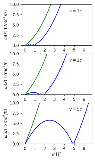
In the first version of [Alperin and Timmermans, 2025] they claimed that allowing \(\gamma^2 <
0\) – i.e. one of the components is attractive – one can realize a roton minimum in
the quasi-particle dispersion relationship, however, the approximation \(c_{a}^2 =
c_{b}^2\) and \(\xi_a^2 = \xi_b\)^2 cannot be realized if \(\gamma^2 < 0\). In particular, if
we take \(g_{a} <0\) to be attractive, then
\[\begin{gather*}
c_{a}^2 = -c^2, \qquad \xi_a^2 = -\xi^2,\\
\omega_{B,a}^2 = -c^2k^2(1-\xi^2k^2), \qquad
\omega_{B,b}^2 = c^2k^2(1+\xi^2k^2).
\end{gather*}\]
The dispersion relation now satisfies
\[\begin{align*}
\abs{\gamma^2}c^4 k^4 &= \bigl((\omega - vk)^2 - \omega_{B,a}^2\bigr)
\bigl((\omega + vk)^2 - \omega_{B,b}^2\bigr),\\
&= \bigl((\omega - vk)^2 + c^2k^2(1-\xi^2k^2)\bigr)
\bigl((\omega + vk)^2 - c^2k^2(1+\xi^2k^2)\bigr),\\
&= (\omega^2 + v^2k^2 - c^2\xi^2k^4)^2
- (c^2k^2 - 2\omega v k)^2.
\end{align*}\]
This has the form
\[\begin{gather*}
\omega^4 + p\omega^2 + q \omega + r = 0, \qquad
p = -2(c^2\xi^2k^4 + v^2k^2), \qquad
q = 4vc^2k^3, \\
r = (v^2k^2 - c^2\xi^2k^4)^2 - c^4k^4
= c^4\xi^4k^8 + (v^4-c^4 - 2v^2c^4\xi^2)k^4
\end{gather*}\]
In the limit of large \(k\) we have
\[\begin{gather*}
p \rightarrow -2 c^2\xi^2k^4, \qquad
q = 4vc^2k^3, \qquad
r \rightarrow c^4\xi^4 k^8,\\
\Delta \rightarrow -c^{12}k^{12}(
512 k^{12}\xi^{12} + 4096k^{6}v^{2}\xi^{6} + 6912v^{4}) < 0\\
\end{gather*}\]
Hence, there are always imaginary frequencies, and the state is unstable.
Old discussion
If we assume \(g_an_a = g_bn_b = gn\), then the linear term vanishes and we have a quadratic
equation in terms of \((\hbar\omega)^2\) that can be easily solved to obtain the following
condition for an instability:
\[\begin{gather*}
(2gn + \tilde{k}^2 - 4\tilde{q}^2)^2 < 4 g_{ab}^{2}n_a n_b.
\end{gather*}\]
We note a couple of points about this result:
The r.h.s. is manifestly non-negative, so there is always an instability since we can
set the l.h.s. to zero by inducing a counterflow with momentum
\[\begin{gather*}
\tilde{q} = \sqrt{\frac{gn}{2} + \frac{\tilde{k}^2}{4}}.
\end{gather*}\]
The physical interpretation is simple: The minimum such \(\tilde{q}\) for \(\tilde{k} =
0\) is the speed of sound
\[\begin{gather*}
\frac{\hbar q}{m} = \sqrt{\frac{gn}{m}} = c.
\end{gather*}\]
Thus, this simply reduces to the Landau criterion for the stability of the
superfluid.
The actual critical velocity is lower due to the interactions \(g_{ab}\):
\[\begin{gather*}
q_{c} = \frac{\sqrt{m\Bigl(gn - \sqrt{g_{ab}^{2}n_a n_b}\Bigr)}}{\hbar}.
\end{gather*}\]
The quasiparticle dispersion has the form:
\[\begin{gather*}
\gamma^2 = \frac{g_{ab}^2}{g_ag_b}, \qquad
g_{ab}^2 n_a n_b = (\gamma gn)^2,\\
(\hbar\omega)^{2} = \tilde{k}^{2}(2gn + \tilde{k}^{2} + 4 \tilde{q}^{2}) \pm
2\tilde{k}^2\sqrt{(2 gn + \tilde{k}^2)4\tilde{q}^2 + \gamma^2(gn)^2}.
\end{gather*} \]
In terms of \(\gamma\), the condition of instability is
\[\begin{gather*}
\Abs{1 + \frac{\tilde{k}^2 - 4\tilde{q}^2}{2gn}} < \abs{\gamma}
\end{gather*}\]
Details
The standard GPE dispersion relationship is
\[\begin{gather*}
\omega^2 = k^2 c^2\Bigl(1 + \frac{\hbar^2 k^2}{2m}\frac{1}{2mc^2}\Bigr)
\end{gather*}\]
which they express below Eq. (7) as \(\omega^2_{B,i} = k^2c_{i}^2(1+\xi_i^2 k^2)\),
which requires
\[\begin{gather*}
c = \sqrt{\frac{gn}{m}}, \qquad \xi = \frac{\hbar}{2mc}.
\end{gather*}\]
This differs from the usual healing length \(h = \sqrt{2} \xi\) where
\[\begin{gather*}
\frac{\hbar^2}{2m h^2} = gn.
\end{gather*}\]
\[\begin{gather*}
(\hbar\omega)^{4}
- 2\tilde{k}^{2}(2gn + \tilde{k}^{2} + 4 \tilde{q}^{2})(\hbar\omega)^{2}+\\
+ 4 (gn)^2 \tilde{k}^{4}
+ 4 gn \tilde{k}^{4} (\tilde{k}^{2} - 4\tilde{q}^{2})
+ \tilde{k}^{8}
- 8 \tilde{k}^{4} \tilde{q}^{2} (\tilde{k}^{2} - 2\tilde{q}^{2})
- 4 g_{ab}^{2}n_a n_b \tilde{k}^{4} = 0,\\
(\hbar\omega)^{2} = \tilde{k}^{2}(2gn + \tilde{k}^{2} + 4 \tilde{q}^{2}) \pm
2\tilde{k}^2\sqrt{8 gn \tilde{q}^2 + 4 \tilde{k}^2 \tilde{q}^2 + g_{ab}^{2}n_a n_b}.
\end{gather*}\]
If the interactions are repulsive, then the discriminant is positive, so we only have an
instability if the \(\omega^2 < 0 \) is negative:
\[\begin{gather*}
(2gn + \tilde{k}^{2} + 4 \tilde{q}^{2})
< 2\sqrt{8 gn \tilde{q}^2 + 4 \tilde{k}^2 \tilde{q}^2 + g_{ab}^{2}n_a n_b},\\
(2gn + \tilde{k}^2 - 4\tilde{q}^2)^2 < 4 g_{ab}^{2}n_a n_b,\\
\end{gather*}\]
To compare with :
\[\begin{align*}
\vect{V}_{j} = \frac{\hbar k_j}{m} &\equiv \pm \frac{\hbar q}{m}\\
\vect{V}_R &\equiv \frac{2\hbar q}{m},\\
\vect{P} &\equiv \hbar k,\\
\gamma &\equiv \frac{g_{ab}}{g} = \frac{g_{ab}}{\sqrt{g_ag_b}}.
\end{align*}\]
\[\begin{gather*}
4\left(\frac{\hbar^2k^2}{4m^2} + \frac{gn}{m}(1-\abs{\gamma}\right) <
\frac{4\hbar^4 k^2q^2}{m^2} <
4\left(\frac{\hbar^2k^2}{4m^2} + \frac{gn}{m}(1+\abs{\gamma}\right)\\
\left(\frac{\hbar^4 k^2q^2}{m^2} - \frac{\hbar^2k^2}{4m^2} - \frac{gn}{m}\right)^2 <
\frac{g_{ab}^2n_an_b}{m^2}.
\end{gather*}\]
For fixed \(\tilde{q}\) we can find the wavevector \(\tilde{k}\) that maximizes the
instability by minimizing the (negative) \((\hbar\omega)^2\):
\[\begin{gather*}
(2gn + 2\tilde{k}^2 + 4\tilde{q}^2)
- 2\sqrt{\cdots} - \frac{2\tilde{k}^2}{\sqrt{\cdots}}(4\tilde{q}^2) = 0\\
(2gn + 2\tilde{k}^2 + 4\tilde{q}^2)\sqrt{\cdots}
= 16 \tilde{q}^2(gn + \tilde{k}^2) + 2g_{ab}^{2}n_a n_b\\
\end{gather*}\]
To simplify these, we define
\[\begin{gather*}
\gamma = \frac{g_{ab}}{\sqrt{g_ag_b}}, \qquad
g_{ab}^2 n_a n_b = (\gamma gn)^2,\\
(\hbar\omega)^{2} = \tilde{k}^{2}(2gn + \tilde{k}^{2} + 4 \tilde{q}^{2}) \pm
2\tilde{k}^2\sqrt{(2 gn + \tilde{k}^2)4\tilde{q}^2 + \gamma^2(gn)^2}.
\end{gather*}\]
\[\begin{gather*}
w^2 = ak + k^2 - 2k\sqrt{qk + b}, \qquad
a = 2gn + 4\tilde{q}^2, \qquad
q = 4\tilde{q}^2, \qquad
b = 8gn\tilde{q}^2 + g_{ab}n_{a}n_{b},\\
(a + 2k) - 2\sqrt{qk + b} - \frac{k}{\sqrt{qk + b}}q = 0\\
(a + 2k)\sqrt{qk + b} = 3qk + 2b\\
(a + 2k)^2(qk + b) = (3qk + 2b)^2\\
4ak^3 + (4b + 2aq - 9q^2)k^2 + (2ab + a^2q - 6qb)k + ba^2 - 4b^2 = 0\\
\end{gather*}\]
This is a rather nasty cubic…
Show code cell content
Hide code cell content
---------------------------------------------------------------------------
KeyboardInterrupt                         Traceback (most recent call last)
Cell In[6], line 9
      5   [k*(k+2*q)+ga*na, gab*nb, -ga*na, -gab*nb],
      6   [gab*na, k*(k-2*q)+gb*nb, -gab*na, -gb*nb],
      7   [ga*na, gab*nb, -(k*(k-2*q)+ga*na), -gab*nb],
      8   [gab*na, gb*nb, -gab*na, -(k*(k+2*q)+gb*nb)]])
----> 9 print(latex(det(M-w*sympy.eye(4)).simplify().collect(w)))

File ~/checkouts/readthedocs.org/user_builds/gpe/conda/latest/lib/python3.14/site-packages/sympy/core/basic.py:1956, in Basic.simplify(self, **kwargs)
   1954 """See the simplify function in sympy.simplify"""
   1955 from sympy.simplify.simplify import simplify
-> 1956 return simplify(self, **kwargs)

File ~/checkouts/readthedocs.org/user_builds/gpe/conda/latest/lib/python3.14/site-packages/sympy/simplify/simplify.py:658, in simplify(expr, ratio, measure, rational, inverse, doit, **kwargs)
    656 expr = _bottom_up(expr, lambda w: getattr(w, 'normal', lambda: w)())
    657 expr = Mul(*powsimp(expr).as_content_primitive())
--> 658 _e = cancel(expr)
    659 expr1 = shorter(_e, _mexpand(_e).cancel())  # issue 6829
    660 expr2 = shorter(together(expr, deep=True), together(expr1, deep=True))

File ~/checkouts/readthedocs.org/user_builds/gpe/conda/latest/lib/python3.14/site-packages/sympy/polys/polytools.py:7363, in cancel(f, _signsimp, *gens, **args)
   7361     if f.is_Number or isinstance(f, Relational) or not isinstance(f, Expr):
   7362         return f
-> 7363     f = factor_terms(f, radical=True)
   7364     p, q = f.as_numer_denom()
   7366 elif len(f) == 2:

File ~/checkouts/readthedocs.org/user_builds/gpe/conda/latest/lib/python3.14/site-packages/sympy/core/exprtools.py:1271, in factor_terms(expr, radical, clear, fraction, sign)
   1269     return rv
   1270 expr2 = sympify(expr)
-> 1271 return do(expr2)

File ~/checkouts/readthedocs.org/user_builds/gpe/conda/latest/lib/python3.14/site-packages/sympy/core/exprtools.py:1261, in factor_terms.<locals>.do(expr)
   1259     # rebuild p not worrying about the order which gcd_terms will fix
   1260     p = Add._from_args(list_args)
-> 1261     p = gcd_terms(p,
   1262         isprimitive=True,
   1263         clear=clear,
   1264         fraction=fraction).xreplace(special)
   1265 elif p.args:
   1266     p = p.func(
   1267         *[do(a) for a in p.args])

File ~/checkouts/readthedocs.org/user_builds/gpe/conda/latest/lib/python3.14/site-packages/sympy/core/exprtools.py:1072, in gcd_terms(terms, isprimitive, clear, fraction)
   1070     terms = sympify(terms)
   1071 terms, reps = mask(terms)
-> 1072 cont, numer, denom = _gcd_terms(terms, isprimitive, fraction)
   1073 numer = numer.xreplace(reps)
   1074 coeff, factors = cont.as_coeff_Mul()

File ~/checkouts/readthedocs.org/user_builds/gpe/conda/latest/lib/python3.14/site-packages/sympy/core/exprtools.py:957, in _gcd_terms(terms, isprimitive, fraction)
    954     cont = cont.gcd(term)
    956 for i, term in enumerate(terms):
--> 957     terms[i] = term.quo(cont)
    959 if fraction:
    960     denom = terms[0].denom

File ~/checkouts/readthedocs.org/user_builds/gpe/conda/latest/lib/python3.14/site-packages/sympy/core/exprtools.py:872, in Term.quo(self, other)
    871 def quo(self, other):  # Term
--> 872     return self.mul(other.inv())

File ~/checkouts/readthedocs.org/user_builds/gpe/conda/latest/lib/python3.14/site-packages/sympy/core/exprtools.py:864, in Term.mul(self, other)
    861 numer = self.numer.mul(other.numer)
    862 denom = self.denom.mul(other.denom)
--> 864 numer, denom = numer.normal(denom)
    866 return Term(coeff, numer, denom)

File ~/checkouts/readthedocs.org/user_builds/gpe/conda/latest/lib/python3.14/site-packages/sympy/core/exprtools.py:558, in Factors.normal(self, other)
    555             else:
    556                 del other_factors[factor]
--> 558 return Factors(self_factors), Factors(other_factors)

File ~/checkouts/readthedocs.org/user_builds/gpe/conda/latest/lib/python3.14/site-packages/sympy/core/exprtools.py:328, in Factors.__init__(self, factors)
    326 if isinstance(factors, Factors):
    327     factors = factors.factors.copy()
--> 328 elif factors in (None, S.One):
    329     factors = {}
    330 elif factors is S.Zero or factors == 0:

File ~/checkouts/readthedocs.org/user_builds/gpe/conda/latest/lib/python3.14/site-packages/sympy/core/numbers.py:1970, in Integer.__eq__(self, other)
   1968 elif isinstance(other, Integer):
   1969     return (self.p == other.p)
-> 1970 return Rational.__eq__(self, other)

File ~/checkouts/readthedocs.org/user_builds/gpe/conda/latest/lib/python3.14/site-packages/sympy/core/numbers.py:1624, in Rational.__eq__(self, other)
   1622 def __eq__(self, other):
   1623     try:
-> 1624         other = _sympify(other)
   1625     except SympifyError:
   1626         return NotImplemented

File ~/checkouts/readthedocs.org/user_builds/gpe/conda/latest/lib/python3.14/site-packages/sympy/core/sympify.py:540, in _sympify(a)
    514 def _sympify(a):
    515     """
    516     Short version of :func:`~.sympify` for internal usage for ``__add__`` and
    517     ``__eq__`` methods where it is ok to allow some things (like Python
   (...)    538
    539     """
--> 540     return sympify(a, strict=True)

File ~/checkouts/readthedocs.org/user_builds/gpe/conda/latest/lib/python3.14/site-packages/sympy/core/sympify.py:422, in sympify(a, locals, convert_xor, strict, rational, evaluate)
    420         conv = _sympy_converter.get(superclass)
    421     if conv is not None:
--> 422         return conv(a)
    424 if cls is type(None):
    425     if strict:

File ~/checkouts/readthedocs.org/user_builds/gpe/conda/latest/lib/python3.14/site-packages/sympy/core/containers.py:337, in <lambda>(d)
    334     __hash__ : Callable[[Basic], Any] = Basic.__hash__
    336 # this handles dict, defaultdict, OrderedDict
--> 337 _sympy_converter[dict] = lambda d: Dict(*d.items())
    339 class OrderedSet(MutableSet):
    340     def __init__(self, iterable=None):

File ~/checkouts/readthedocs.org/user_builds/gpe/conda/latest/lib/python3.14/site-packages/sympy/core/containers.py:267, in Dict.__new__(cls, *args)
    265 else:
    266     raise TypeError('Pass Dict args as Dict((k1, v1), ...) or Dict({k1: v1, ...})')
--> 267 elements = frozenset(items)
    268 obj = Basic.__new__(cls, *ordered(items))
    269 obj.elements = elements

File ~/checkouts/readthedocs.org/user_builds/gpe/conda/latest/lib/python3.14/site-packages/sympy/core/containers.py:110, in Tuple.__hash__(self)
    107         return super().__ne__(other)
    108     return self.args != other
--> 110 def __hash__(self):
    111     return hash(self.args)
    113 def _to_mpmath(self, prec):

KeyboardInterrupt:
Dynamics Response
We now consider driving the system where \(V(x, t) = V_0 \cos(\omega t)\cos(kx) =
\tfrac{1}{2}V_0(e^{\omega t/\I} + e^{-\omega t/\I})\cos(kx)\) is small. This
adds an inhomogeneous term which we treat as the same order a \(\epsilon_{\pm}\):
\[\begin{gather*}
\begin{pmatrix}
\op{H} + n_0\mathcal{E}'' - \hbar \omega & n_0\mathcal{E}''\\
n_0\mathcal{E}'' & \op{H}^* + n_0\mathcal{E}'' + \hbar \omega^*
\end{pmatrix}
\begin{pmatrix}
\epsilon_+(x) \\
\epsilon_-^*(x)
\end{pmatrix}
=
-\frac{V_0}{2}\cos(kx)
\begin{pmatrix}
\psi_0\\
\psi_0^*
\end{pmatrix},
\end{gather*}\]
the formal solution of which can be found by inverting the matrix.
Homogeneous Matter
The full linear response follows from inverting the matrix, but we need to be a bit
careful. We start by setting \(k_0 = 0\) so that parity is conserved. Then we expand:
\[\begin{gather*}
\psi = \sqrt{n_0}\Bigl(
1 + (\epsilon_{+}e^{-\I\omega t} + \epsilon_{-}e^{\I\omega t})\cos(kx)\Bigr),\\
n = n_0 + \sqrt{n_0}\cos(kx)2\Re\Bigl(
\epsilon_{+}e^{-\I\omega t} + \epsilon_{-}e^{\I\omega t}\Bigr)
\end{gather*}\]
Collecting all terms, we have two independent sets of equations:
\[\begin{gather*}
\begin{pmatrix}
A - \hbar\omega e^{\I\eta} & B\\
B & A + \hbar\omega e^{-\I\eta}
\end{pmatrix}
\begin{pmatrix}
\epsilon_{+}\\
\epsilon_{-}^*
\end{pmatrix}
=
-\frac{V_0\sqrt{n_0}}{4}
\begin{pmatrix}
1\\
1
\end{pmatrix},\\
A = H_0 + B, \qquad
B = n_0\mathcal{E}''(n_0).
\end{gather*}\]
\[\begin{gather*}
\begin{pmatrix}
\epsilon_{+}\\
\epsilon_{-}^*
\end{pmatrix}
=
-\frac{V_0\sqrt{n_0}}{4\Bigl(
(A - \hbar\omega e^{\I\eta})(A + \hbar\omega e^{-\I\eta}) - B^2
\Bigr)}
\begin{pmatrix}
A + \hbar\omega e^{-\I\eta} & -B\\
-B & A - \hbar\omega e^{\I\eta}
\end{pmatrix}
\begin{pmatrix}
1\\
1
\end{pmatrix},\\
=
-\frac{V_0\sqrt{n_0}}{4\Bigl(
A^2 - \hbar^2\omega^2 - B^2 - 2\I A\hbar\omega \sin(\eta)
\Bigr)}
\begin{pmatrix}
A + \hbar\omega e^{-\I\eta} -B\\
A - \hbar\omega e^{\I\eta} - B
\end{pmatrix},\\
\epsilon_{+} =
-\frac{V_0\sqrt{n_0}(A + \hbar\omega e^{-\I\eta} -B)}{4\Bigl(
A^2 - \hbar^2\omega^2 - B^2 - 2\I A\hbar\omega \sin(\eta)\Bigr)}\\
\epsilon_{-} =
-\frac{V_0\sqrt{n_0}(A - \hbar\omega e^{\I\eta} - B)}{4\Bigl(
A^2 - \hbar^2\omega^2 - B^2 - 2\I A\hbar\omega \sin(\eta)\Bigr)},\\
\epsilon_{+} =
-\frac{V_0\sqrt{n_0}(A + \hbar\omega e^{-\I\eta} -B)}{4\Bigl(
A^2 - \hbar^2\omega^2 - B^2 - 2\I A\hbar\omega \sin(\eta)\Bigr)}\\
\epsilon_{-} =
-\frac{V_0\sqrt{n_0}(A - \hbar\omega e^{\I\eta} - B)}{4\Bigl(
A^2 - \hbar^2\omega^2 - B^2 - 2\I A\hbar\omega \sin(\eta)\Bigr)}
\end{gather*}\]
\[\begin{split}
\begin{pmatrix}
\op{H} + g n_0 & g\psi_0^2\\
g \bar{\psi}_0^2 & \bar{\op{H}} + g n_0
\end{pmatrix}\cdot
\begin{pmatrix}
u(x)\\
v(x)
\end{pmatrix}
=
\omega
\begin{pmatrix}
\mat{1} \\
& -\mat{1}
\end{pmatrix}\cdot
\begin{pmatrix}
u(x)\\
v(x)
\end{pmatrix},
\end{split}\]
where \(n_0 = \abs{\psi_0}^2\) and \(\op{H} = -\hbar^2\nabla^2/2m + gn_0 + \op{V}_{\text{ext}}\) is the single-particle Hamiltonian for the ground state. To solve this numerically, we write this as \(\mat{A}\cdot\vect{q} = \omega \mat{B}\cdot\vect{q}\).
These matrices have the following properties: \(\mat{A} = \mat{A}^\dagger\) and \(\mat{B} = \mat{B}^\dagger\) are Hermitian, and the matrix \(\mat{C} = \mat{C}^{-1} = \bigl(\begin{smallmatrix}&\mat{1}\\\mat{1}\end{smallmatrix}\bigr)\) conjugates \(\mat{A}\):
\[\begin{split}
\mat{C}\cdot\mat{A}\cdot\mat{C} = \bar{\mat{A}}\\
\mat{C}\cdot\mat{B}\cdot\mat{C} = -\bar{\mat{B}}.
$$. Thus, if we have one eigenvalue $\omega_{+}$ and eigenvector $\vect{q}_{+}$, then, we must have another pair $\omega_{-} = \bar{\omega}_{+}$ and $\vect{q}_{-} = \mat{C}\cdot\bar{\vect{q}}_{+}$:\end{split}\]
\mat{A}\vect{q}{+} = \omega+ \mat{B}\vect{q}{+}\
\bar{\mat{A}}\mat{C}\vect{q}{+} = \omega_+ \bar{\mat{B}}\mat{C}\vect{q}_{+}.
$$
Furthermore, if \(\psi_0\) is a stationary state, then \(\op{H}\psi_0 = \mu\psi_0\).
One has two choices: solve the non-symmetric eigenvalue problem \((\mat{B}^{-1}\cdot\mat{A})\cdot\vect{q} = \omega\vect{q}\), or try to massage this into a form where \(\mat{B}\) is positive definite.
\[
(\mat{A} + 2\mat{1})\cdot\vect{q} = (\omega\mat{B} + 2\mat{I})\cdot\vect{q}
\]