import mmf_setup;mmf_setup.nbinit()
%pylab inline --no-import-all
This cell adds /home/docs/checkouts/readthedocs.org/user_builds/gpe/checkouts/latest/src to your path, and contains some definitions for equations and some CSS for styling the notebook. If things look a bit strange, please try the following:
- Choose "Trust Notebook" from the "File" menu.
- Re-execute this cell.
- Reload the notebook.
%pylab is deprecated, use %matplotlib inline and import the required libraries.
Populating the interactive namespace from numpy and matplotlib
Utils#
This notebook describes some of the utilities provided here.
Periodic Potential Extension#
A common case is that of a large trap along the \(x\) direction where we are interested in the behavior near the center. To enable this case, we provide a flag cells_x which allows the user to specify a small number of \(k_r\) cells near the center of the trap to simulate. To avoid numerical issues at the boundaries, we need a transformation so that the potential can be applied in such a way as to be \(C_{\infty}\) periodic over this new interval. There are several options:
Harmonic Potentials#
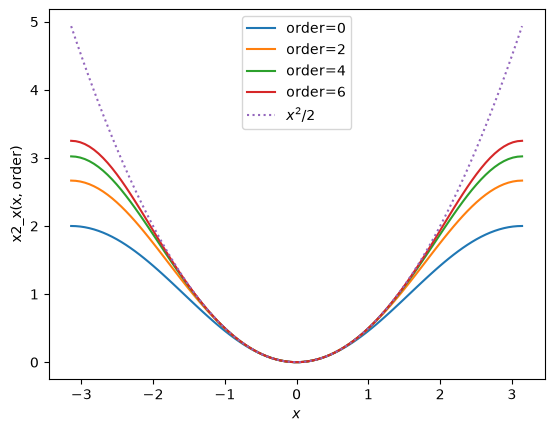
If the potential is Harmonic \(V(x) \propto x^2\), then we can replace it with a periodic function that matches near the center. This is done by the function gpe.utils.x2_2() which is a periodic function \(f(x)\) with period \(2\pi\) approximating \(x^2/2\) at the center:
from gpe.utils import x2_2

x = np.linspace(-np.pi, np.pi, 100)
for order in [0,2,4,6]:
    plt.plot(x, x2_2(x, order=order), label="order={}".format(order))
plt.plot(x, x**2/2, ':', label="$x^2/2$", scaley=False)
plt.legend(); plt.xlabel('$x$'); plt.ylabel('x2_x(x, order)')
[I 20:02:20 numexpr.utils] NumExpr defaulting to 2 threads.
[I 20:02:20 root] Patching zope.interface.document.asReStructuredText to format code
Text(0, 0.5, 'x2_x(x, order)')
Abscissa Transform#
Another option is to transform the abscissa so as to render the potential periodic. If \(V(x) = V(-x)\), then the following transform works quite nicely, rendering the potential periodic over the interval \(x\in [-1,1]\):
import gpe.utils;reload(gpe.utils)
from gpe.utils import x_periodic

def V(x):
    return x**2/2

def Vp(x, x0, p=3):
    xt = x_periodic(x, x0=x0, p=p)
    return V(xt)

x = np.linspace(-1, 1, 100)
for x0 in [0.8, 0.9, 1.0]:
    plt.plot(x, Vp(x, x0=x0, p=3), label="x0={}".format(x0))
plt.plot(x, V(x), ':', label="$V(x)$", scaley=False)
plt.legend(); plt.xlabel('$x$'); plt.ylabel('V(x, p)')
---------------------------------------------------------------------------
NameError                                 Traceback (most recent call last)
Cell In[3], line 1
----> 1 import gpe.utils;reload(gpe.utils)
      2 from gpe.utils import x_periodic
      3
      4 def V(x):

NameError: name 'reload' is not defined
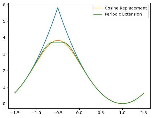
Here is a comparison of the two methods with the default values (chosen to match roughly):
from gpe.utils import x2_2, x_periodic


w = 1.5
m = 2.3
L = 3.0

def V(x):
    return m*(w*x)**2/2

def Vp1(x):
    k = 2*np.pi/L
    return m*w**2/k**2 * x2_2(k*x)

def Vp2(x):
    xt = L/2*x_periodic(2*x/L)
    return V(xt)

x = np.linspace(-L/2, L/2, 100)

# This is the transform which shifts the potential to
# be centered at x0
x0 = 1.0
x_ = (x - x0 - x.min()) % L + x.min()
plt.plot(x, V(x_))
plt.plot(x, Vp1(x_), label="Cosine Replacement")
plt.plot(x, Vp2(x_), label="Periodic Extension")
plt.legend()
<matplotlib.legend.Legend at 0x7f03efe9f230>
        Lx = self._get_Lx(state)
        xyz[0] = (x - self.get('x0', t_=t_) - x.min()) % Lx + x.min()
        return xyz
---------------------------------------------------------------------------
NameError                                 Traceback (most recent call last)
Cell In[5], line 1
----> 1 Lx = self._get_Lx(state)
      2 xyz[0] = (x - self.get('x0', t_=t_) - x.min()) % Lx + x.min()
      3 return xyz

NameError: name 'self' is not defined