import mmf_setup; mmf_setup.nbinit()
import os, sys
from pathlib import Path
FIG_DIR = Path(mmf_setup.ROOT) / '../Docs/_build/figures/'
os.makedirs(FIG_DIR, exist_ok=True)
import logging; logging.getLogger("matplotlib").setLevel(logging.CRITICAL)
%matplotlib
import numpy as np, matplotlib.pyplot as plt
try: from myst_nb import glue
except: glue = None

from matplotlib.animation import FuncAnimation
from gpe.contexts import FPS

$\newcommand{\vect}[1]{\mathbf{#1}} \newcommand{\uvect}[1]{\hat{#1}} \newcommand{\abs}[1]{\lvert#1\rvert} \newcommand{\norm}[1]{\lVert#1\rVert} \newcommand{\I}{\mathrm{i}} \newcommand{\ket}[1]{\left|#1\right\rangle} \newcommand{\bra}[1]{\left\langle#1\right|} \newcommand{\braket}[1]{\langle#1\rangle} \newcommand{\Braket}[1]{\left\langle#1\right\rangle} \newcommand{\op}[1]{\mathbf{#1}} \newcommand{\mat}[1]{\mathbf{#1}} \newcommand{\d}{\mathrm{d}} \newcommand{\D}[1]{\mathcal{D}[#1]\;} \newcommand{\pdiff}[3][]{\frac{\partial^{#1} #2}{\partial {#3}^{#1}}} \newcommand{\diff}[3][]{\frac{\d^{#1} #2}{\d {#3}^{#1}}} \newcommand{\ddiff}[3][]{\frac{\delta^{#1} #2}{\delta {#3}^{#1}}} \newcommand{\floor}[1]{\left\lfloor#1\right\rfloor} \newcommand{\ceil}[1]{\left\lceil#1\right\rceil} % The following allows KaTeX to render these for significantly improved % performance on CoCalc. \newcommand{\DeclareMathOperator}[2]{\newcommand{#1}{#2}} \DeclareMathOperator{\Tr}{Tr} \DeclareMathOperator{\erf}{erf} \DeclareMathOperator{\erfi}{erfi} \DeclareMathOperator{\sech}{sech} \DeclareMathOperator{\sn}{sn} \DeclareMathOperator{\cn}{cn} \DeclareMathOperator{\dn}{dn} \DeclareMathOperator{\sgn}{sgn} \DeclareMathOperator{\order}{O} \DeclareMathOperator{\diag}{diag} % \newcommand{\mylabel}[1]{\label{#1}\tag{#1}} \newcommand{\degree}{\circ}$

This cell adds /home/docs/checkouts/readthedocs.org/user_builds/gpe/checkouts/latest/src to your path, and contains some definitions for equations and some CSS for styling the notebook. If things look a bit strange, please try the following:

• Choose "Trust Notebook" from the "File" menu.
• Re-execute this cell.
• Reload the notebook.

Using matplotlib backend: module://matplotlib_inline.backend_inline

Harmonic Traps

Harmonically trapped gases play a special role in cold atom physics for several reasons.

1. All potentials look harmonic close to their minimum. Thus, a laser with a gaussian intensity profile can be used to make a harmonic close to the core:

   \[\begin{gather*} V(x) = V_0 e^{-x^2/2\sigma^2} = V_0\left( 1 - \frac{x^2}{2\sigma^2} + \frac{x^4}{8\sigma^4} + \cdots\right). \end{gather*}\]

   Identifying the second term with a harmonic trapping potential gives

   \[\begin{gather*} V_0 = -m\omega^2\sigma^2, \qquad V(x) = \text{const} + \frac{m\omega^2}{2}x^2 - \underbrace{\frac{m\omega^2 x^4}{8\sigma^2}}_{\frac{m^2\omega^4 x^4}{8V_0}} + \cdots, \end{gather*}\]

   where the last term characterizes the anharmonicities.

2. Aspects of dynamics are after simple in harmonic traps due to the fact that all classical trajectories have the same period. This leads to many cases where the shape of a trapped gas remains invariant, simply oscillating and vibrating with the trapping frequencies. See for example [Castin and Dum, 1996] where the effects of harmonic traps can be incorporated into scaled coordinates and phases – see Dynamically Rescaled GPE (dr-GPE) which make use of to model cloud expansion for imaging,

3. Related is Kohn’s Harmonic theorem (see [Wu and Zaremba, 2014] for details) which basically says that, no matter what the internal interactions are, the center of mass of a harmonically trapped cloud will follow the classical trajectory of a particle with the total mass of the system.

Here we will demonstrate some of these effects as realized in the GPE.

Show code cell source

Hide code cell source

from gpe.bec import _StateBase, GPEMixin, HOMixin
from gpe import utils
from gpe.minimize import MinimizeState


# Note: StateBase is earlier in the mro, spoiling the ability to set g in StateHOMixin
@utils._GPU.add_non_GPU_methods
class State(GPEMixin, HOMixin, utils.StateWithExperimentMixin, _StateBase):
    def __init__(self, *v, g, ws, **kw):
        self.g = g
        self.ws = ws
        return super().__init__(*v, **kw)
    
    def shift(self, x0):
        """Shift the wavefunction by x0.  Relies on fourier basis."""
        kx = self.basis.kx
        self.set_psi(
            self.basis.ifft(
                np.exp(1j*kx*x0) * self.basis.fft(self.get_psi(), axis=0), axis=0))

    def get_Vext_GPU(self, state=None):
        if state is None:
            state = self
        x = state.xyz[0] 
        Vext = (sum(state.m*(w*x)**2/2 for w, x in zip(state.ws, state.xyz))
                - state.m*state.ws[0]**2*x**4/8/self.experiment.sigma)
        if state.initializing:
            Vext -= self.mu
            
        return Vext

        
class Experiment(utils.ExperimentBase):
    m = hbar = 1
    ws = 2*np.pi * np.array([1 , 3, 5])
    healing_length = 0.1
    Rx_x_TF = 2.0
    Rperp_perp_TF = 1.3
    dx_healing_length = 0.5
    n0 = 1.0
    State = State
    t_unit = 1
    dim = 1
    sigma = np.inf  # Anisotropy parameter - width of gaussian.
    
    def init(self):
        dx = self.dx_healing_length * self.healing_length
        mu = self.hbar**2 / 2 / self.m / self.healing_length**2
        wx = self.ws[0]
        xyz_TF = np.sqrt(2*mu / self.m) / self.ws
        Lx = 2 * self.Rx_x_TF * xyz_TF[0]
        Lyz = 2 * self.Rperp_perp_TF * xyz_TF[1:]
        Lxyz = [Lx] + list(Lyz)
        Lxyz = Lxyz[:self.dim]
        Nxyz = [utils.get_good_N(L/dx) for L in Lxyz]
        
        g = mu / self.n0
        self.state_args = dict(
            experiment=self,
            hbar=self.hbar,
            m=self.m,
            g=g,
            mu=mu,
            ws=self.ws,  # Maybe should delegate?
            Nxyz=Nxyz,
            Lxyz=Lxyz)
        super().init()
        
    # We should provide a default in ExperimentBase
    def get_state(self):
        return self.State(**self.state_args)
        
    def get_initial_state(self):
        s = self.get_state()
        m = MinimizeState(s)
        psi0 = m.minimize(use_scipy=True).get_psi()
        s = self.get_state()
        s.set_psi(psi0)
        s.pre_evolve_hook()
        return s
    

e = Experiment()
s = e.get_state()
s0 = e.get_initial_state()
s.plot(label="TF");
s0.plot(label="Ground State");

[I 03:36:46 root] Patching zope.interface.document.asReStructuredText to format code
[I 03:36:46 numexpr.utils] NumExpr defaulting to 2 threads.

/home/docs/checkouts/readthedocs.org/user_builds/gpe/checkouts/latest/src/gpe/bec.py:1112: RuntimeWarning: divide by zero encountered in log10
  ir, uv = map(np.log10, self.get_convergence())

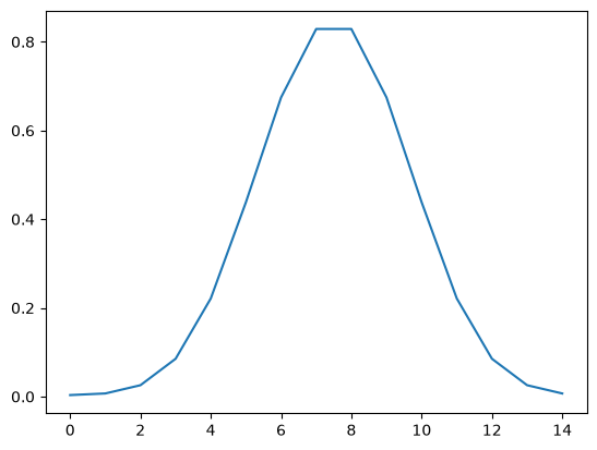
We first plot the initial states to make sure we have a large enough box. Now we shift the state to the right and watch it oscillate.

Show code cell source

Hide code cell source

from gpe.contexts import FPS
from pytimeode.evolvers import EvolverABM

e = Experiment()
s = e.get_initial_state()
s.shift(1)
T = 4*e.t_unit
Nt = 100
dT = T/Nt
dt = 0.4*s.t_scale
steps = int(np.ceil(dT/dt))
dt = dT/steps
ev = EvolverABM(s, dt=dt)
fig, ax = plt.subplots()
Es = [s.get_energy()]
for f in FPS(Nt, fig=fig, embed=True):
    ev.evolve(steps)
    s = ev.y
    Es.append(s.get_energy())
    V = s.get_Vext()
    ax.cla()
    ev.y.plot(fig=fig)
    ax.set(ylim=(0, 1.2))
    ax.plot(s.x, V/V.max())
assert np.allclose(Es, Es[0])

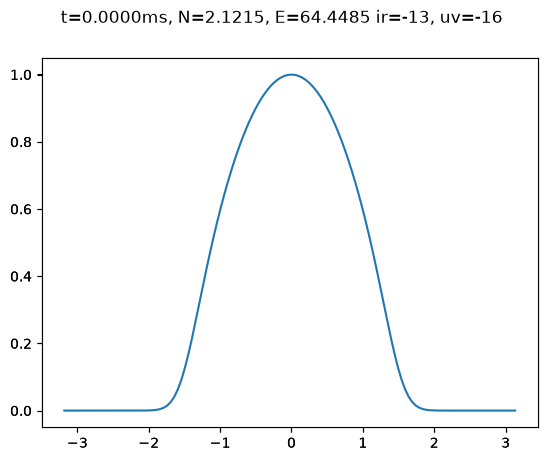
Notice that the oscillations preserve the shape. The is a feature of harmonic traps that follows from Kohn’s Harmonic Trapping theorem (see [Wu and Zaremba, 2014] and references therein for details). We now show that this also applies in higher dimension by solving a 2D problem:

Show code cell source

Hide code cell source

from gpe.contexts import FPS
from pytimeode.evolvers import EvolverABM

e = Experiment(dim=2)
s = e.get_initial_state()
s.shift(1)
T = 1*e.t_unit
Nt = 100
dT = T/Nt
dt = 0.2*s.t_scale
steps = int(np.ceil(dT/dt))
dt = dT/steps
ev = EvolverABM(s, dt=dt)
fig, axs = plt.subplots(2, 1, figsize=(10,5))
axs = s.plot(axs=axs)
Es = [s.get_energy()]
for f in FPS(Nt, fig=fig, embed=True):
    ev.evolve(steps)
    [ax.cla() for ax in axs]
    Es.append(ev.y.get_energy())
    ev.y.plot(axs=axs)
assert np.allclose(Es, Es[0])

The bottom frame shows the evolution of the wavefunction phase. Notice that the contours remain linear and equally spaced – this indicates that the velocity of the cloud is constant, hence the motion is shape preserving.

Anharmonicities

Here is what happens if we add a slight anharmonicity:

Show code cell source

Hide code cell source

e = Experiment(sigma=10)
s = e.get_initial_state()
s.shift(1)
T = 4*e.t_unit
Nt = 100
dT = T/Nt
dt = 0.4*s.t_scale
steps = int(np.ceil(dT/dt))
dt = dT/steps
ev = EvolverABM(s, dt=dt)
fig, ax = plt.subplots()
Es = [s.get_energy()]
for f in FPS(Nt, fig=fig, embed=True):
    ev.evolve(steps)
    s = ev.y
    Es.append(s.get_energy())
    V = s.get_Vext()
    ax.cla()
    ev.y.plot(fig=fig)
    ax.set(ylim=(0, 1.2))
    ax.plot(s.x, V/V.max())
assert np.allclose(Es, Es[0])

Now the cloud has some internal oscillations.

Thomas Fermi Approximation

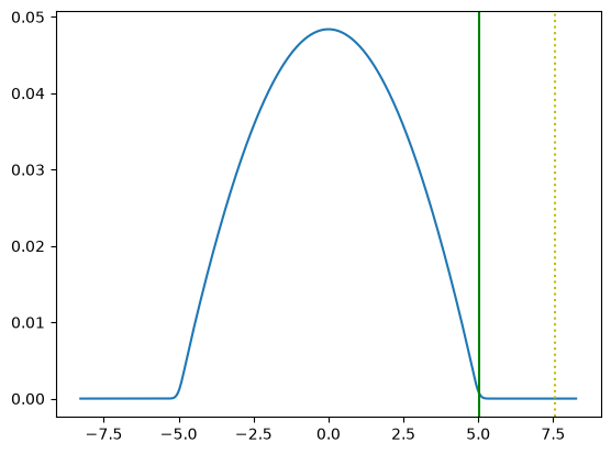
e = Experiment(dim=2, healing_length=0.1/4, ws=2*np.pi * np.array([1, 200, 5]),
              Rx_x_TF=1.3, Rperp_perp_TF=2.5)
s = e.get_initial_state()
mu = (s.braket(s.get_Hy(subtract_mu=False)) / s.braket(s)).real
plt.plot(s.x, s.get_density_x())
wx, wy = s.ws[:2]
x_TF0 = np.sqrt(2*mu/s.m)/wx
x_TF1 = np.sqrt(2*(mu-s.hbar*(wx+wy)/2)/s.m)/wx
plt.axvline([x_TF0], c='y', ls=':')
plt.axvline([x_TF1], c='g', ls='-')

<matplotlib.lines.Line2D at 0x7c68fbf786e0>

plt.plot(s.get_density()[s.basis.Nxyz[0]//2, :])

[<matplotlib.lines.Line2D at 0x7c68fbc31fd0>]