Show code cell source

Hide code cell source

import mmf_setup
mmf_setup.nbinit()
%pylab inline --no-import-all

$\newcommand{\vect}[1]{\mathbf{#1}} \newcommand{\uvect}[1]{\hat{#1}} \newcommand{\abs}[1]{\lvert#1\rvert} \newcommand{\norm}[1]{\lVert#1\rVert} \newcommand{\I}{\mathrm{i}} \newcommand{\ket}[1]{\left|#1\right\rangle} \newcommand{\bra}[1]{\left\langle#1\right|} \newcommand{\braket}[1]{\langle#1\rangle} \newcommand{\Braket}[1]{\left\langle#1\right\rangle} \newcommand{\op}[1]{\mathbf{#1}} \newcommand{\mat}[1]{\mathbf{#1}} \newcommand{\d}{\mathrm{d}} \newcommand{\D}[1]{\mathcal{D}[#1]\;} \newcommand{\pdiff}[3][]{\frac{\partial^{#1} #2}{\partial {#3}^{#1}}} \newcommand{\diff}[3][]{\frac{\d^{#1} #2}{\d {#3}^{#1}}} \newcommand{\ddiff}[3][]{\frac{\delta^{#1} #2}{\delta {#3}^{#1}}} \newcommand{\floor}[1]{\left\lfloor#1\right\rfloor} \newcommand{\ceil}[1]{\left\lceil#1\right\rceil} % The following allows KaTeX to render these for significantly improved % performance on CoCalc. \newcommand{\DeclareMathOperator}[2]{\newcommand{#1}{#2}} \DeclareMathOperator{\Tr}{Tr} \DeclareMathOperator{\erf}{erf} \DeclareMathOperator{\erfi}{erfi} \DeclareMathOperator{\sech}{sech} \DeclareMathOperator{\sn}{sn} \DeclareMathOperator{\cn}{cn} \DeclareMathOperator{\dn}{dn} \DeclareMathOperator{\sgn}{sgn} \DeclareMathOperator{\order}{O} \DeclareMathOperator{\diag}{diag} % \newcommand{\mylabel}[1]{\label{#1}\tag{#1}} \newcommand{\degree}{\circ}$

This cell adds /home/docs/checkouts/readthedocs.org/user_builds/gpe/checkouts/latest/src to your path, and contains some definitions for equations and some CSS for styling the notebook. If things look a bit strange, please try the following:

• Choose "Trust Notebook" from the "File" menu.
• Re-execute this cell.
• Reload the notebook.

%pylab is deprecated, use %matplotlib inline and import the required libraries.
Populating the interactive namespace from numpy and matplotlib

DVR (from mmfutils)

Here we discuss some of the bases provided in mmfutils.math.bases for representing problems with rotational symmetry such a cylindrical and spherical symmetry. We discuss a general set of Bessel-function DVR bases for representing the radial wavefunction of “spherically” symmetric problems in \(d\) spatial dimensions (\(d=2\) for cylindrical symmetry and \(d=3\) for spherical symmetry), as well as a simplified basis for spherically symmetric problems where we represent the radial wavefunction on a periodic lattice. This latter basis allows us to perform operations such as convolution.

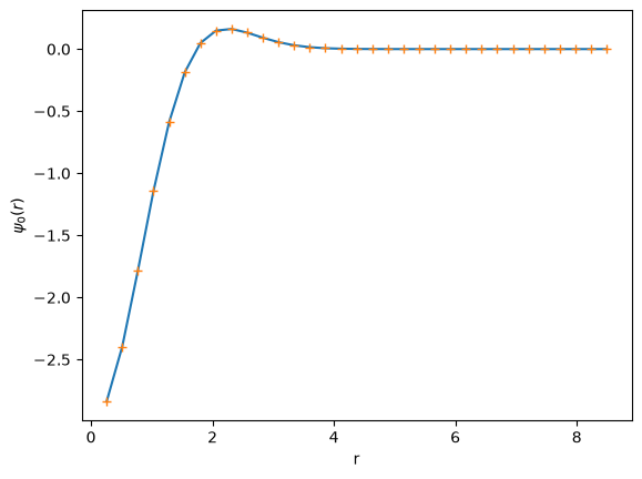
Here is a quick demonstration, using these bases to solve for the eigenstates of the spherical harmonic oscillator:

\[\begin{gather*} V(r) = \frac{m\omega^2r^2}{2}, \qquad E_n = \hbar\omega(n+\tfrac{d}{2}). \end{gather*}\]

Spherical Basis

\[\begin{gather*} \psi_0(r) = Ae^{-r^2/2a_0^2}, \qquad \nabla^2 \psi = \frac{1}{r^{d-1}} \pdiff{}{r}\left(r^{d-1}\pdiff{\psi(r)}{r}\right) = \frac{r^2 - a_0^2 d}{a_0^4}\psi_0(r) \end{gather*}\]

from mmfutils.math import bases

eps = np.finfo(float).eps
hbar = m = w = 1
a0 = np.sqrt(hbar / m / w)
R = np.sqrt(-2 * a0**2 * np.log(eps))
k_max = np.sqrt(-np.log(eps) / a0**2)
N = int(np.ceil(k_max * 2 * R / np.pi))

d = 3
basis = bases.SphericalBasis(N=N, R=R)

r = basis.xyz[0]
psi0 = np.exp(-((r / a0) ** 2) / 2)
ax = plt.subplot(111)
ax.plot(r, basis.laplacian(psi0))
ax.plot(r, (r**2 - a0**2 * d) / a0**4 * psi0, "+")
ax.set(xlabel="r", ylabel=r"$\psi_0(r)$");

[I 03:36:27 root] Patching zope.interface.document.asReStructuredText to format code
[I 03:36:27 numexpr.utils] NumExpr defaulting to 2 threads.

Background

Here are the properties of the basis, including abscissa, basis functions, integration weights, and some quantities that appear in the DVR literature. The general idea of a DVR basis is to introduce a set of basis functions \(F_n(x) = \braket{x|F_n}\) and an associated set of abscissa \(x_n\) such that:

\[\begin{gather*} \newcommand{\vect}[1]{\vec{#1}} F_{m}(x_n) \propto \delta_{mn}. \tag{locality} \end{gather*}\]

These bases are generalized version of the Dirac delta function \(\delta(x-x_n) = \braket{x|x_n}\) restricted to a limited set of momenta with maximum momentum \(k\):

\[\begin{gather*} \ket{F_n} \propto \ket{\Delta_n} = \op{P}_{k}\ket{x_n}, \qquad \op{P}_k = \int_{p<k}\ket{p}\bra{p}, \qquad \op{P}_k^2 = \op{P}_k. \end{gather*}\]

A challenge is to choose a consistent set of abscissa so that these functions are orthogonal:

\[\begin{gather*} \braket{\Delta_m|\Delta_n} = \braket{x_m|\Delta_n} = \Delta_n(x_m) = \frac{\delta_{mn}}{\lambda_n}. \end{gather*}\]

The actual basis functions differ in their normalization so that they are orthonormal:

\[\begin{gather*} \braket{F_m|F_n} = \delta_{mn} = \lambda_n\braket{\Delta_m|\Delta_n}, \qquad \ket{F_n} = \sqrt{\lambda_n}\ket{\Delta_n}, \qquad \lambda_n = \frac{1}{\braket{\Delta_n|\Delta_n}} = \frac{1}{\Delta_n(x_n)} = \frac{1}{F_n^2(x_n)},\qquad F_n(x_m) = \frac{\delta_{mn}}{\sqrt{\lambda_n}}. \end{gather*}\]

The normalization factors \(\lambda_n\) act as a set of integration weights that are exact for all functions \(g(x) = F_{i}^*(x) F_{j}(x)\) expressed as products of basis elements:

\[\begin{gather*} \int g(x) = \sum_n \lambda_n g(x_n), \qquad g(x) = F_{i}(x)^* F_{j}(x). \end{gather*}\]

These weights can thus be used to effectively compute quantities such as the total particle number by integrating \(n(x) = \psi^*(x)\psi(x)\).

This condition ensures that if the wavefunction \(\psi(r)\) mostly lies in the subspace spanned by the basis, it can be expanded by simply evaluating it at the abscissa:

\[\begin{gather*} \braket{F_n|\psi} = \int F_{n}^*(r) \psi(r) \approx \sum_m \sqrt{\lambda_m}\psi(r_m) \int F_{n}^*(r)F_m(r) = \sum_m \sqrt{\lambda_m}\psi(r_m) \underbrace{ \sum_j \lambda_j \overbrace{F_n^*(r_j)F_m(r_j)} ^{\delta_{nj}\delta_{mj}/\sqrt{\lambda_n^*\lambda_m}} }_{\delta_{mn}} = \sqrt{\lambda_n}\psi(r_n). \end{gather*}\]

The coefficients can thus be computed by simply evaluating the wavefunction at the abscissa:

\[\begin{gather*} \psi(r) = \sum_n f_n F_n(r), \qquad f_n = \sqrt{\lambda_n}\psi(r_n). \end{gather*}\]

The key utility of these bases is that one can obtain exponentially accurate representations if with a tabulated kinetic energy operator, while simply evaluating the potential at the abscissa:

\[\begin{gather*} K_{mn} = \Braket{F_m|\op{K}|F_n}, \qquad V_{mn} = \braket{F_m|\op{V}|F_n} \approx \delta_{mn}V(r_n). \end{gather*}\]

In general, choosing a consistent set of basis functions and abscissa is a challenge, and most (all?) known examples are based on some form of orthogonal polynomial.

Sinc-Function Basis

Here we demonstrate these properties with the sinc-function basis with equally spaced abscissa \(x_n\):

(4)\[\begin{gather} \DeclareMathOperator{\sinc}{sinc} \ket{\Delta_n} = \op{P}_k\ket{x_n}, \qquad \op{P}_k = \int_{p<k} \frac{\d{p}}{2\pi}\ket{p}\bra{p}, \\ \Delta_n(x) = \braket{x|\Delta_n} = \int_{-k}^{k} \frac{\d{p}}{2\pi}e^{\I p (x-x_n)} = \frac{k}{\pi}\sinc \bigl(k(x-x_n)\bigr) \\ x_n = x_0 + an, \qquad z_n = kx_n = k x_0 + \pi n, \qquad a = \frac{\pi}{k} \tag{abscissa} \\ \lambda_n = \braket{\Delta_n|\Delta_n}^{-1} = \frac{1}{\Delta_n(x_n)} = \frac{1}{F_n^2(x_n)} = a \tag{weights} \\ F_n(x) = \sqrt{\lambda_n}\Delta_n(x) = \frac{\sinc \bigl(k(x-x_n)\bigr)}{\sqrt{a}} \tag{basis functions} \\ \op{T}_{mn} = \Bigl\langle F_m\Big|-\diff[2]{}{x}\Big|F_n\Bigr\rangle = \frac{1}{a^2}\begin{cases} 2(-1)^{m-n}/(m-n)^2 & m \neq n,\\ \pi^2/3 & m = n. \end{cases}\tag{kinetic term} \end{gather}\]

Spherical Symmetry

Recall that in \(d\)-dimensions, the Laplacian is:

\[\begin{gather*} \nabla^2 = \Delta^{\mathbb{R}^{d}} = r^{1-d}\pdiff{}{r}r^{d-1}\pdiff{}{r} + \frac{1}{r^2}\Delta_{S^{d-1}} \end{gather*}\]

where \(\Delta_{S^{d-1}}\) is the Laplacian suitably restricted to the sphere \(S^{d-1}\) (i.e. the Laplace–Beltrami operator. Expressing the wavefunction in terms of “spherical” harmonics \(Y_l^m(\uvect{x})\), one has:

\[\begin{gather*} \Delta_{S^{d-1}}Y_l^m(\uvect{x}) = -l(l+d-2)Y_l^m(\uvect{x}). \end{gather*}\]

The wavefunction can thus be expressed in terms of the following basis:

\[\begin{gather*} \psi(\vect{x}) = \frac{1}{r^{(d-1)/2}}u(r)Y_l^m(\uvect{x}), \end{gather*}\]

such that the radial wavefunction \(u(r)\) satisfies:

\[\begin{gather*} \nabla^2\psi(r, \Omega) = \frac{Y_l^m(\uvect{x})}{r^{(d-1)/2}}\left[ \diff[2]{}{r} - \frac{\nu_{d,l}^2 - 1/4}{r^2} \right]u(r), \qquad \nu_{d,l} = l + \frac{d}{2} - 1. \end{gather*}\]

The Bessel-function DVR basis is chosen to provide an exponentially accurate representation of the radial portion of the wavefunction, including the singular centrifugal piece. Thus, the DVR basis functions are orthogonal under the metric:

\[\begin{gather*} \braket{F_{\nu,m}|F_{\nu,n}} = \int_0^{\infty} \d{r}\; F_{\nu,m}^*(r)F_{\nu,n}(r) = \delta_{mn}, \end{gather*}\]

which does not include the angular or \(r^{d-1}\) factors. The advantage of this is exponential accuracy for analytic potentials, but each \(\nu_{d,l}\) has a different set of abscissa which is inconvenient. We have found that fairly good accuracy can be achieved using only \(l=0\) and \(l=1\) bases, shifting the residual portion of the \(r^{-2}\) term into the potential, but this needs to be carefully checked. (For example, with \(d=3\), the \(l=0\) basis works well for even \(l\) while the \(l=1\) basis must be used for odd \(l\).)

Cylindrical Basis

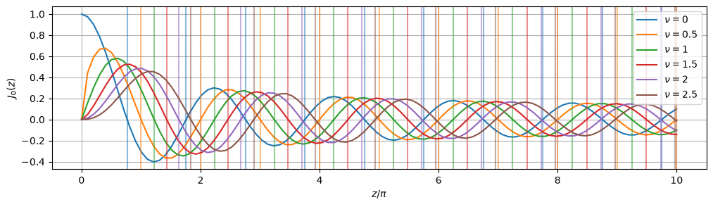
To represent problems with cylindrical coordinates we use a periodic basis for \(x\) and a Bessel-function DVR basis for the radial coordinate. Here we describe the properties of the Bessel-function basis for the radial direction. These are expressed in terms of the Bessel functions (with \(n \equiv \alpha \equiv \nu\)):

\[\begin{gather*} J_\nu(r) = \frac{1}{\pi}\int_0^{\pi}\cos(\nu\tau - r\sin\tau)\d{\tau} - \frac{\sin \nu\pi}{\pi}\int_0^\infty e^{-r\sinh t - \nu t}\d{t}, \end{gather*}\]

which satisfy the following useful relationships:

\[\begin{gather*} \int_0^{\infty} \d{r}\; r J_{\nu}(ur)J_{\nu}(vr) = \frac{1}{u}\delta(u-v),\\ \int_0^{\infty}\frac{\d{r}}{r}\; J_{\alpha}(r)J_{\beta}(r) = \frac{2}{\pi}\frac{\sin\Bigl(\tfrac{\pi}{2}(\alpha-\beta)\Bigr)}{\alpha^2-\beta^2}. \end{gather*}\]

import numpy as np
from scipy.integrate import quad
from mmfutils.math import bessel

alpha = 1.1
beta = 1.2
x = 1.5
J_alpha = bessel.J(alpha, 0)
J_beta = bessel.J(beta, 0)


def J(x, nu):
    """Integral definition of J_n(x)."""

    def integrand1(tau):
        return np.cos(nu * tau - x * np.sin(tau)) / np.pi

    def integrand2(t):
        return np.sin(nu * np.pi) * np.exp(-x * np.sinh(t) - nu * t) / np.pi

    res1, err1 = quad(integrand1, 0, np.pi)
    with np.errstate(over="ignore"):
        # Ignore harmless overflow errors
        res2, err2 = quad(integrand2, 0, np.inf)
    return res1 - res2, np.sqrt(err1**2 + err2**2)


assert np.allclose(J(x, alpha)[0], J_alpha(x))


def i2(x):
    return J_alpha(x) * J_beta(x) / x


res, err = quad(i2, 0, np.inf, epsabs=0.001)
exact = 2 / np.pi * np.sin(np.pi / 2 * (alpha - beta)) / (alpha**2 - beta**2)
assert np.allclose(exact, res, atol=err)

%pylab inline --no-import-all
plt.figure(figsize=(12, 3))
z = np.linspace(1e-12, 10 * np.pi, 100)
for nu in [0, 0.5, 1, 1.5, 2, 2.5]:
    (l,) = plt.plot(z / np.pi, bessel.J(nu, d=0)(z), label=r"$\nu={}$".format(nu))
    for z0 in bessel.j_root(nu, 10):
        if z0 <= z.max():
            plt.axvline(z0 / np.pi, c=l.get_c(), ls="-", alpha=0.5)
plt.grid(True)
plt.legend()
plt.xlabel(r"$z/\pi$")
plt.ylabel(r"$J_0(z)$")

%pylab is deprecated, use %matplotlib inline and import the required libraries.
Populating the interactive namespace from numpy and matplotlib

Text(0, 0.5, '$J_0(z)$')

There is a separate basis for each value of \(\nu\) which handles a different angular-momentum singularity. Once this is fixed, the basis functions are:

\[\begin{gather*} \nu = l+\frac{d}{2}-1,\\ J_\nu(k r_n) = 0, \qquad z_n = k r_n, \tag{abscissa}\\ F_{\nu,n}(r) = (-1)^{n+1}\frac{\sqrt{2k}H_{\nu,n}(k r)}{1+r/r_n}, \qquad H_{\nu,n}(z) = \frac{\sqrt{z} J_\nu(z)}{z-z_n}, \tag{basis functions} \\ \lambda_n = \frac{1}{F_{\nu,n}(r_n)^2} = \frac{2}{k z_n [J_\nu'(z_n)]^{2}} \tag{weights}\\ [\mat{T}]_{mn} = \Biggl\langle F_{\nu,m}\Bigg|-\diff[2]{}{r}+\frac{\nu^2-\tfrac{1}{4}}{r^2} \Bigg|F_{\nu,n}\Biggr\rangle = k^2\begin{cases} (-1)^{m-n}\frac{8z_mz_n}{(z_m^2 - z_n^2)^2} & n \neq m\\ \tfrac{1}{3}\left[1 + \frac{2(\nu^2 - 1)}{z_n^2}\right] & n = m \end{cases}, \tag{kinetic term} \end{gather*}\]

For use with wavefunctions, we must include the transformation to and from

from mmfutils.math.bases import CylindricalBasis
basis = CylindricalBasis(Nxr=(2, 10), Lxr=(1.0, 1.0))
x, r = basis.xyz
k_x, k_r = basis.k_max

Line-of-Sight Integrals

For visualization, it is often desired to express a density in terms of the line-of-sight integrals, for example, when imaging a cylindrically symmetric atomic cloud. The formal definitions are:

\[\begin{align*} \newcommand{\d}{\mathrm{d}} \newcommand{\abs}[1]{{\lvert#1\rvert}} \d{r} &= \frac{y\d{y} + z\d{z}}{r}\\ n_{1D} &= \iint_{-\infty}^\infty \d{y}\d{z}\; n(r) = \int_0^{\infty} \d{r}\; 2\pi r n(r),\\ n_{2D}(y) &= \int_{-\infty}^\infty \d{z}\; n(r) %= 2\int_{0}^\infty \d{z}\; n\left(\sqrt{y^2+z^2}\right) = 2\int_{\abs{y}}^{\infty} \d{r}\; \frac{rn(r)}{\sqrt{r^2-y^2}}. \tag{Abel Transform} \end{align*}\]

The first of these is easy to implement because of the properties of the basis. Recall that if \(f(r)\) and \(g(r)\) are well represented in the basis, that the integral \(\int_0^{\infty}\d{r}\; f^*(r)g(r) = \sum_n\lambda_n f^*(r_n)g(r_n)\) is accurate. This means that if the wavefunction

\[\begin{gather*} \psi(r) = \frac{u(r)}{\sqrt{r}} \end{gather*}\]

is well represented, then the integral

\[\begin{gather*} \int_0^\infty\d{r}\; \abs{u(r)}^2 = \int_0^\infty\d{r}\; r\abs{\psi(r)}^2 = \frac{n_{1D}}{2\pi} \approx \sum\lambda_n \abs{u(r_n)}^2 = \sum\lambda_n r_nn(r_n) \end{gather*}\]

is accurate. This is computed by integrate1 in the code.

The second implements an Abel Transform, which is more complicated. If high accuracy is needed, then we can do the following integrals manually, and use the resulting matrix to compute the transform, but this is very slow.

\[\begin{gather*} n(r) \approx \sum_{mn} \psi_{m}^*\psi_{n} \frac{F_m(r)F_n(r)}{r}\\ n_{2D}(y) \approx \sum_{mn} \psi_{m}^*\psi_{n} \int_{\abs{y}}^{\infty}\d{r}\; \frac{2F_m(r)F_n(r)}{\sqrt{r^2-y^2}}. \end{gather*}\]

Instead, we simply use the form:

\[\begin{gather*} n_{2D}(y) = \int_{-\infty}^{\infty} \d{z}\; n\left(\sqrt{z^2+y^2}\right). \end{gather*}\]

We use the basis to extrapolate the wavefunction to the desired abscissa, and then use a trapazoidal rule along \(z\) to compute the integral. This can be broadcast to perform reasonably efficiently.

For testing, consider a Gaussian:

\[\begin{gather*} n(x, r) = e^{-(x^2+r^2)/r_0^2}, \\ n_{2D}(x,y) = \sqrt{\pi}r_0e^{-(x^2+y^2)/r_0^2}, \qquad n_{1D}(x) = \pi r_0^2e^{-x^2/r_0^2}. \end{gather*}\]

Another test:

\[\begin{gather*} n(x, r) = r^2 e^{-(x^2+r^2)/r_0^2}, \\ n_{2D}(x,y) = \frac{\sqrt{\pi}r_0(r_0^2+2y^2)}{2}e^{-(x^2+y^2)/r_0^2}, \qquad n_{1D}(x) = \pi r_0^4e^{-x^2/r_0^2}. \end{gather*}\]

%pylab inline --no-import-all
import numpy as np
from mmfutils.math.bases import CylindricalBasis
from mmfutils.math.bases.tests import test_bases

basis = CylindricalBasis(Nxr=(64, 32), Lxr=(25.0, 5.0))
x, r = basis.xyz
Ny = 50
ys = np.linspace(0, r.max(), Ny)[None, :]
r0 = 1.2

n = np.exp(-(x**2 + r**2) / r0**2)
n_1D = np.pi * r0**2 * np.exp(-(x**2) / r0**2)
n_2D = np.sqrt(np.pi) * r0 * np.exp(-(x**2 + ys**2) / r0**2)

print(
    "{}% max error".format(100 * abs(basis.integrate2(n, y=ys) - n_2D).max() / n_2D.max())
)

n = r**2 * np.exp(-(x**2 + r**2) / r0**2)
n_1D = np.pi * r0**4 * np.exp(-(x**2) / r0**2)
n_2D = np.sqrt(np.pi) * r0 / 2 * (r0**2 + 2 * ys**2) * np.exp(-(x**2 + ys**2) / r0**2)

print(
    "{}% max error".format(100 * abs(basis.integrate2(n, y=ys) - n_2D).max() / n_2D.max())
)

%pylab is deprecated, use %matplotlib inline and import the required libraries.
Populating the interactive namespace from numpy and matplotlib

---------------------------------------------------------------------------
ModuleNotFoundError                       Traceback (most recent call last)
Cell In[6], line 4
      1 get_ipython().run_line_magic('pylab', 'inline --no-import-all')
      2 import numpy as np
      3 from mmfutils.math.bases import CylindricalBasis
----> 4 from mmfutils.math.bases.tests import test_bases
      5 
      6 basis = CylindricalBasis(Nxr=(64, 32), Lxr=(25.0, 5.0))
      7 x, r = basis.xyz

ModuleNotFoundError: No module named 'mmfutils.math.bases.tests'

Harmonic Oscillator

Here we check the basis for a 2D Harmonic oscillator. The exact results are:

\[\begin{gather*} E_n = \hbar \omega (n + 1). \end{gather*}\]

The ground state wave-function is:

\[\begin{gather*} \psi(r) \propto e^{-r^2/2a_0^2}, \qquad \psi_k \propto e^{-k^2a_0^2}, \qquad a_0 = \sqrt{\frac{\hbar}{m\omega}}. \end{gather*}\]

from mmfutils.math.bases import CylindricalBasis

eps = np.finfo(float).eps
hbar = m = w = 1
a0 = np.sqrt(hbar / m / w)
R = np.sqrt(-2 * a0**2 * np.log(eps))
k_max = np.sqrt(-np.log(eps) / a0**2)
Nr = int(np.ceil(k_max * 2 * R / np.pi))

basis = CylindricalBasis(Nxr=(1, Nr), Lxr=(1.0, R))


def get_V(r):
    return m * w**2 * r**2 / 2


Vs = []
Ks = []
Hs = []
Es = []
for l in range(4):
    r = basis._r(Nr, l=l)
    V = get_V(r)
    K = basis._get_K(l=l)[0]  # Without factors of sqrt(r)
    H = K / 2 + np.diag(V)
    assert np.allclose(H, H.T.conj())
    E = np.linalg.eigvalsh(H)
    Vs.append(V)
    Ks.append(K)
    Hs.append(H)
    Es.append(E)

Es_ = sorted(sum((E.tolist() for E in Es), []))

l = 3
l0 = 1
nu0 = basis.nu(l=l0)
nu = basis.nu(l=l)

r = basis._r(Nr, l=l0)
K = basis._get_K(l=l0)[0]  # Without factors of sqrt(r)

V = get_V(r) + (nu**2 - nu0**2) / r**2 * hbar**2 / 2 / m
H = K / 2 + np.diag(V)
assert np.allclose(H, H.T.conj())
E = np.linalg.eigvalsh(H)
E

array([ 4.        ,  6.        ,  8.        , 10.        , 12.        ,
       14.        , 16.        , 18.        , 20.        , 22.00000001,
       24.0000003 , 26.00000489, 28.00006078, 30.00057424, 32.00407358,
       34.02130778, 36.08128298, 38.23022802, 40.50974723, 42.94011599,
       45.52473409, 48.26031172, 51.14238164, 54.16702739, 57.33112378,
       60.63269981, 64.072669  , 67.68788588, 71.56379868, 73.68477758,
       76.84257618, 83.21411642, 93.85473386])

Spherical Basis

For spherically symmetric problems, one solution is to use a Bessel function DVR basis.

Here we check the basis for a 3D Harmonic oscillator. The exact results are:

\[\begin{gather*} E_n = \hbar \omega (n + \tfrac{3}{2}). \end{gather*}\]

The ground state wave-function is:

\[\begin{gather*} \psi(r) \propto e^{-r^2/2a_0^2}, \qquad \psi_k \propto e^{-k^2a_0^2}, \qquad a_0 = \sqrt{\frac{\hbar}{m\omega}}. \end{gather*}\]

from mmfutils.math.bases import SphericalBasis

eps = np.finfo(float).eps
hbar = m = w = 1
a0 = np.sqrt(hbar / m / w)
R = np.sqrt(-2 * a0**2 * np.log(eps))
k_max = np.sqrt(-np.log(eps) / a0**2)
Nr = int(np.ceil(k_max * 2 * R / np.pi))

basis = SphericalBasis(N=Nr, R=R)

def get_V(r):
    return m * w**2 * r**2 / 2


Vs = []
Ks = []
Hs = []
Es = []
for l in range(4):
    r = basis.xyz[0]
    V = get_V(r)
    K = basis._get_K(l=l)[0]  # Without factors of sqrt(r)
    H = K / 2 + np.diag(V)
    assert np.allclose(H, H.T.conj())
    E = np.linalg.eigvalsh(H)
    Vs.append(V)
    Ks.append(K)
    Hs.append(H)
    Es.append(E)

Es_ = sorted(sum((E.tolist() for E in Es), []))

---------------------------------------------------------------------------
AttributeError                            Traceback (most recent call last)
Cell In[10], line 12
      8 Es = []
      9 for l in range(4):
     10     r = basis.xyz[0]
     11     V = get_V(r)
---> 12     K = basis._get_K(l=l)[0]  # Without factors of sqrt(r)
     13     H = K / 2 + np.diag(V)
     14     assert np.allclose(H, H.T.conj())
     15     E = np.linalg.eigvalsh(H)

AttributeError: 'SphericalBasis' object has no attribute '_get_K'

Another possibility is to use a periodic 1D basis of odd functions. This follows from the radial equations:

\[\begin{gather*} \nabla^2 \psi(\vect{r}) = \frac{1}{r^2}\diff{}{r} r^2 \diff{\psi}{r}, \qquad \psi(r) = u(r)/r,\qquad \nabla^2 \psi(r) = \nabla^2 \frac{u(r)}{r} = \frac{1}{r}\diff[2]{u(r)}{r}. \end{gather*}\]

Hence, we can work with the radial Schrödinger equation for \(u(r)\) instead (but still use the proper functions to compute the non-linear pieces).

Fourier Transforms

The Fourier transform simplifies by noting that \(\tilde{n}(\vect{k}) = \tilde{n}(k)\) depends only on the magnitude of \(\vect{k}\) so we can take \(\vect{k} = (0,0,k)\):

\[\begin{gather*} \tilde{n}(k) = \int \d^3{\vect{r}}\; e^{-\I\vect{k}\cdot\vect{r}} n(r)\\ = 2\pi \int_0^{\infty}r^2\d{r}\int_{-1}^{1}\d\cos\theta\; e^{-\I kr\cos\theta} n(r) = 2\pi \int_0^{\infty}r^2\d{r}\; 2\frac{\sin kr}{kr} n(r) = \frac{4\pi}{k} \int_0^{\infty}\d{r}\; r\sin(kr) n(r)\\ = \frac{2\pi}{k} \int_{-\infty}^{\infty}\d{x}\; x\sin(kx)n(\abs{x}) = \frac{-2\pi}{k} \Im \int_{-\infty}^{\infty}\d{x}\; e^{-\I kx} xn(\abs{x}). \end{gather*}\]

Hence, we can use the standard 1D Fourier transform of \(rn(\abs{r})\). The only subtlety is at \(k=0\) where we can use:

\[\begin{gather*} \tilde{n}(0) = \int_0^{\infty}\d{r}\; 4\pi r^2 n(r) = \int_{-\infty}^{\infty}\d{x}\; 2\pi x^2 n(\abs{x}). \end{gather*}\]

The inverse is similar with some factors of \(2\pi\):

\[\begin{gather*} n(r) = \frac{1}{\pi r} \int_{0}^{\infty}\frac{\d{k}}{2\pi}\; \sin(kr) k\tilde{n}(\abs{k}) = \frac{1}{2\pi r} \Im \int_{-\infty}^{\infty}\frac{\d{k}}{2\pi}\; e^{\I kr} k\tilde{n}(\abs{k}), \qquad n(0) = \int_{0}^{\infty}\frac{\d{k}}{(2\pi)^3} 4\pi k^2 \tilde{n}(k). \end{gather*}\]

As an example, we use the proton form factor with \(r_0^{-2} = k_0^2 = 0.71\)GeV\(^2\):

\[\begin{gather*} G_p(r) = \frac{e^{-r/r_0}}{8\pi r_0^3}, \qquad \tilde{G}_{p}(k) = \left(1 + \frac{k^2}{k_0^2}\right)^{-2} \end{gather*}\]

import numpy as np

r_0 = 1.0
k_0 = 1.0 / r_0

N = 64
L = 10.0
# L = 10.0
dx = L / N
dk = 2 * np.pi / L


######## To Do: Make work with symmetric lattice!
symmetric = True  # If True, then use a symmetric grid with no point at x=0
symmetric = False
x = np.arange(N) * dx - L / 2 + (dx / 2 if symmetric else 0)
k = 2 * np.pi * np.fft.fftfreq(N, dx)
r = abs(x)

G_r = np.exp(-r / r_0) / 8 / np.pi * r_0**3
G_k = 1.0 / (1 + k**2 / k_0**2) ** 2


def sft(n, dx=dx):
    """Spherical Fourier transform"""
    if symmetric:
        assert np.allclose(n, n[::-1])
    else:
        assert np.allclose(n[1:], n[1:][::-1])

    N = len(n)
    L = dx * N
    x = np.arange(N) * dx - L / 2.0 + (dx / 2 if symmetric else 0)
    k = 2 * np.pi * np.fft.fftfreq(N, dx)
    _ft = np.fft.fft(np.fft.fftshift(x * n))
    # assert np.allclose(_ft.real, 0)
    return np.ma.divide(-2 * np.pi * _ft.imag * dx, k).filled(
        (2 * np.pi * x**2 * n * dx).sum()
    )


def isft(n, dx=dx):
    """Spherical Inverse Fourier transform"""
    N = len(n)
    L = dx * N
    dk = 2 * np.pi / L
    x = np.arange(N) * dx - L / 2.0 + (dx / 2 if symmetric else 0)
    k = 2 * np.pi * np.fft.fftfreq(N, dx)
    _ift = np.fft.fftshift(np.fft.ifft(k * n))
    # assert np.allclose(_ft.real, 0)
    return np.ma.divide(_ift.imag, 2 * np.pi * dx * x).filled(
        (2 * np.pi * k**2 * n / (2 * np.pi) ** 3).sum() * dk
    )

Coulomb Convolution

One problem that arises in some nuclear physics work is to compute the Coulomb potential for a nucleus:

\[\begin{gather*} V(R) = \int \d^3{\vect{r}}\; \frac{n(r)}{4\pi\abs{r-R}}. \end{gather*}\]

This has two complications: 1) the singularities and the 2) long-range nature of the interaction which can give rise to images in a periodic box. Our standard resolution is to use the truncated interaction and pad the array of charges so that the convolution with the truncated interaction does not pickup charges from the neighboring cells (which are now further away because of the padding).

\[\begin{gather*} K_D(r) = \begin{cases} \frac{1}{4\pi r} & r\leq D,\\ 0 & r> D. \end{cases}, \qquad \tilde{K}_{D}(k) = \frac{1-\cos kD}{k^2}, \qquad \tilde{K}_{D}(0) = \frac{D^2}{2}. \end{gather*}\]

def pad(f):
    N = len(f)
    F = np.zeros(2 * N, dtype=f.dtype)
    F[N // 2 : N // 2 + N] = f
    F[-N // 2] = f[0]
    return F


def unpad(F):
    N = len(F) // 2
    return F[N // 2 : N // 2 + N]

import scipy.special

sp = scipy
eps = np.finfo(float).eps
a = 0.5
D = L
n_r = np.exp(-(r**2) / 2 / a**2)
V_r = a**3 / (r + eps) * np.sqrt(np.pi / 2) * sp.special.erf((r + eps) / a / np.sqrt(2))

_K = 2 * np.pi * np.fft.fftfreq(2 * N, dx)
K_D = np.ma.divide(1.0 - np.cos(_K * D), _K**2).filled(D**2 / 2.0)
res = unpad(isft(sft(pad(n_r)) * K_D))
assert np.allclose(res, V_r)

# Self-contained convolution.  Reduces some intermediate steps.
def coulomb(n_r, dx=dx):
    N = len(n_r)
    L = N * dx
    D = L

    X = np.arange(2 * N) * dx - L
    K = 2 * np.pi * np.fft.fftfreq(2 * N, dx)

    K_D = np.ma.divide(1.0 - np.cos(K * D), K**2).filled(D**2 / 2.0)
    n = pad(n_r)

    _ft = np.fft.fft(np.fft.fftshift(X * n))
    tmp = np.ma.divide(-_ft.imag, K).filled((X**2 * n).sum()) * K_D
    _ift = np.fft.fftshift(np.fft.ifft(K * tmp))
    dk = np.pi / L
    res = np.ma.divide(_ift.imag, X).filled((K**2 * tmp / (2 * np.pi)).sum() * dk * dx)

    return unpad(res)


assert np.allclose(coulomb(n_r), V_r)

# Now get rid of fftshift.
def coulomb(n_r, dx=dx):
    N = len(n_r)
    L = N * dx
    D = L
    dk = np.pi / L

    X = np.arange(2 * N) * dx - L
    K = 2 * np.pi * np.fft.fftfreq(2 * N, dx)

    K_D = np.ma.divide(1.0 - np.cos(K * D), K**2).filled(D**2 / 2.0)
    n = pad(n_r)

    _ft = np.fft.fft(X * n)
    tmp = np.ma.divide(-_ft.imag, K).filled((X**2 * n).sum()) * K_D
    _ift = np.fft.ifft(-_ft.imag * K_D)
    res = np.ma.divide(_ift.imag, X).filled(-(K**2 * tmp / (2 * np.pi)).sum() * dk * dx)
    # Not sure I understand the - sign needed here...

    return unpad(res)


assert np.allclose(coulomb(n_r), V_r)

Discrete Sine Transform

We can improve performance here by using the discrete sine transform (DST). For best performance, one should use the DST-II or RODFT10 version which computes:

(5)\[\begin{gather} \DeclareMathOperator{\DST}{DST} 2N f_n = \overbrace{2\sum_{k=0}^{N-1} F_k \sin[\pi(k+\tfrac{1}{2})(n+1)/N] \Big|_{n=0}^{N-1}}^{\DST_{II}(F_k)}, \tag{RODFT10 (DST-II)}\\ F_k = \overbrace{(-1)^{k}f_{N-1}+2\sum_{n=0}^{N-2} f_n \sin[\pi(k+\tfrac{1}{2})(n+1)/N] \Big|_{k=0}^{N-1}}^{\DST_{III}(f_x)}, \tag{RODFT10 (DST-III)}\\ \DST_{III}^{-1} = \frac{1}{2N}\DST_{II}. \end{gather}\]

In physical notation, we have abscissa \(x = x_n = (n+1) R/N\) and \(k = k_n = \pi (n+1/2)/R = 2\pi (n+1/2)/L\) for \(n\in\{0,1,\cdots, N-1\}\). Note that here we have \(N\) points in the radial direction with radius \(R\), hence \(\d{x} = R/N\). The correspondance with the usual periodic box is \(L = 2R\).

\[\begin{gather*} 2Nf_x = \overbrace{2\sum_k F_{k}\sin(kx)}^{\DST_{II}[F_k]} = 2R\int_0^{\infty} \frac{\d{k}}{\pi} F_{k} \sin(kx),\\ F_k = \overbrace{\cdots + 2\sum_x f_x \sin(kx)}^{\DST_{III}[f_x]} = \cdots + \frac{2N}{R}\int_0^{\infty} \d{x}\;f_x \sin(kx),\\ \int_0^{\infty}\frac{\d{k}}{\pi} F_{k} \sin(kx) \equiv \frac{1}{2R}\DST_{II}[F_k] \equiv \frac{N}{R}\DST_{III}^{-1}[F_k],\\ \int_0^{\infty} \d{x}\;f_x \sin(kx) \equiv \frac{R}{2N}{\DST_{III}[f_x]}. \end{gather*}\]

From these and the expressions derived earlier, we can express the full 3D Fourier transforms:

\[\begin{gather*} \tilde{f}_k = \frac{4\pi}{k} \int_{0}^{\infty}\d{x}\; \sin(kx) xf(x) = \frac{2\pi}{k}\frac{R}{N}\DST_{III}[x f(x)],\\ f(x) = \frac{1}{2\pi x} \int_0^{\infty}\frac{\d{k}}{\pi}\; \sin(kx) k \tilde{f}_k = \frac{1}{2\pi x}\frac{N}{R}\DST_{III}^{-1}[k \tilde{f}_k]. \end{gather*}\]

Convolution (3D)

Convolution of spherically symmetric functions proceeds as follows:

\[\begin{gather*} \DeclareMathOperator{\DST}{DST} V(x) = \int \d^{3}\vect{r}\;C(\norm{\vect{x}-\vect{r}})y(r) = \int \frac{\d^{3}\vect{k}}{(2\pi)^3}\; e^{\I \vect{k}\cdot\vect{r}} \tilde{C}_{\vect{k}} \tilde{y}_{\vect{k}} = \int \frac{\d^{3}\vect{k}}{(2\pi)^3}\; e^{\I \vect{k}\cdot\vect{r}} \tilde{C}_{\vect{k}} \tilde{y}_{\vect{k}},\\ \tilde{C}_{\vect{k}} = \frac{4\pi}{k} \int_0^{\infty}\d{r}\; \sin(kr) rC(r) = \begin{cases} \frac{2\pi}{k} \frac{R}{N}\DST(rC) & k \neq 0\\ \int \d^3{\vect{r}}\;C(r) & k = 0. \end{cases} \end{gather*}\]

\[\begin{gather*} V(r) = \frac{1}{2\pi r}\frac{N}{R} \DST^{-1}\left[ k \tilde{C}_k \tilde{y}_k \right] = \frac{1}{2\pi x}\frac{N}{R} \DST^{-1}\left[ k \tilde{C}_k \frac{2\pi}{k} \frac{R}{N} \DST(ry_r) \right] = \frac{1}{r} \DST^{-1}\left[\tilde{C}_k \DST(ry_r)\right]. \end{gather*}\]

This is the form used in SphericalBasis.convolve().

%pylab inline --no-import-all
import scipy.fftpack
import scipy as sp


def dst(f):
    return scipy.fftpack.dst(f, type=3)


def idst(F):
    N = len(F)
    return scipy.fftpack.dst(F, type=2) / (2.0 * N)


# Now work it for only positive abscissa
N = 32
R = 5.0
dx = R / N
r = (1.0 + np.arange(N)) * dx
rr = np.linspace(0, R, 100)
k = np.pi * (0.5 + np.arange(N)) / R

a = 0.5

n_r = np.exp(-(r**2) / 2 / a**2)
V_r = a**3 / r * np.sqrt(np.pi / 2) * sp.special.erf(r / a / np.sqrt(2))

f_r = r * n_r
f_rr = rr * np.exp(-(rr**2) / 2 / a**2)
df_r = (1.0 - (r / a) ** 2) * np.exp(-(r**2) / 2 / a**2)
df_rr = (1.0 - (rr / a) ** 2) * np.exp(-(rr**2) / 2 / a**2)
ddf_r = (r**2 - 3 * a**2) / a**4 * f_r
ddf_rr = (rr**2 - 3 * a**2) / a**4 * f_rr

assert np.allclose(idst(-(k**2) * dst(f_r)), ddf_r)

F_k = dst(f_r) / (2.0 * N)
assert np.allclose(
    f_rr, 2 * (F_k[None, :] * np.sin(k[None, :] * rr[:, None])).sum(axis=-1)
)

%pylab is deprecated, use %matplotlib inline and import the required libraries.
Populating the interactive namespace from numpy and matplotlib

Finally, we compute the convolution required for the Coulomb potential. These relationships are much simpler:

\[\begin{gather*} k\tilde{n}(k) = 4\pi \int_0^{\infty}\d{r}\; \sin(kr) rn(r), \qquad V(r) = \frac{1}{\pi r} \int_{0}^{\infty}\frac{\d{k}}{2\pi}\; \sin(kr) k\tilde{n}(k) \end{gather*}\]

Again, we do this in a padded box:

We use the following test functions (in \(d\)-dimensions):

\[\begin{gather*} y(r) = A e^{-(r/r_0)^2/2}, \qquad \nabla^2 y(r) = \frac{r^2 - d r_0^2}{r_0^4} y(r), \qquad e^{a\nabla^2} y(r) = A\frac{r_0^d}{\sqrt{r_0^2+2a}^d} e^{-r^2/(r_0^2+2a)/2}. \end{gather*}\]

As a test, the convolution of this Gaussian with itself in 3D is:

\[\begin{gather*} \int \d^{3}\vect{r}\; y(\norm{\vect{x}-\vect{r}})y(r) = 2\pi\int_0^{\infty}\d{r}\int_{-1}^{1}\d{\cos\theta}\; r^2 y\left(\sqrt{x^2 + r^2 - 2xr\cos\theta}\right)y(r)\\ = A^2r_0^3 \pi^{3/2}e^{-(x/r_0)^2/4} \end{gather*}\]

# Now work it for only positive abscissa
L = 2 * R
D = L

rN_r = np.concatenate([r * n_r, 0 * n_r])
K = np.pi * (0.5 + np.arange(2 * N)) / (2 * R)

K_D = np.ma.divide(1.0 - np.cos(K * D), K**2).filled(D**2 / 2.0)

kN_k = dst(rN_r)
V = idst(K_D * kN_k)[:N] / r
assert np.allclose(V, V_r)

Here we check that convolution preserves the norm. We use the proton form factor.

import scipy.fftpack


def dst(f):
    return scipy.fftpack.dst(f, type=3)


def idst(F):
    N = len(F)
    return scipy.fftpack.dst(F, type=2) / (2.0 * N)


N = 32
R = 5.0
r0 = 0.5
k0 = 10.0
dx = R / N
r = (1.0 + np.arange(N)) * dx
k = np.pi * (0.5 + np.arange(N)) / R

metric = 4 * np.pi * r**2 * dx
n = np.exp(-((r / r0) ** 2) / 2) / (r0 * np.sqrt(2 * np.pi)) ** 3
assert np.allclose(1, (n * metric).sum())

Gk = 1.0 / (1 + k**2 / k0**2) ** 2
G = idst(Gk) / r
q = idst(Gk * dst(r * n)) / r

assert np.allclose(1, (q * metric).sum())

Convolution proceedes as follows (let \(q = \sqrt{r^2 + R^2 - 2rR\cos\theta}\) so that \(q\d{q} = -rR\d(\cos\theta)\)):

\[\begin{gather*} V(R) = \int\d^{3}{r}\; n(r)f(\abs{R-r}) = \frac{2\pi}{R} \int_{0}^{\infty}\d{r}\; rn(r) \int_{\abs{R-r}}^{\abs{R+r}}\d{q}\; qf(q) = \frac{\pi}{R} \int_{-\infty}^{\infty}\d{r}\; rn(\abs{r}) \int_{\abs{R-r}}^{\abs{R+r}}\d{q}\; qf(q) \end{gather*}\]

Bessel Function DVR

To implement the spherical and cylindrical DVR bases, we need some numerical code for evaluating Bessel functions. These are provided by the module mmfutils.math.bessel, some of which we describe here.

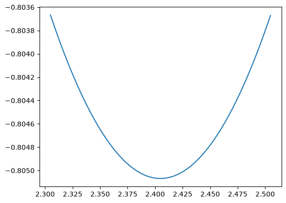
J_sqrt_pole

For evaluating the basis functions, we need the function \(F(z)\):

\[\begin{gather*} F(z) = \frac{f(z)}{z - z_n} = \frac{\sqrt{z}J_{\nu}(z)}{z - z_n},\qquad F'(z) = \frac{f'(z)}{z - z_n} - \frac{f(z)}{(z - z_n)^2}. \end{gather*}\]

%pylab inline --no-import-all
from importlib import reload
from mmfutils.math import bessel

reload(bessel)

nu = 0.0
n = 0

zn = bessel.j_root(nu=nu, N=n + 1)[n]
zn = zn
F = bessel.J_sqrt_pole(nu=nu, zn=zn, d=0)
dF = bessel.J_sqrt_pole(nu=nu, zn=zn, d=1)
z = np.linspace(zn - 0.1, zn + 0.1, 1000)
plt.plot(z, F(z))

zn

%pylab is deprecated, use %matplotlib inline and import the required libraries.
Populating the interactive namespace from numpy and matplotlib

np.float64(2.404825557695773)

Interpolation

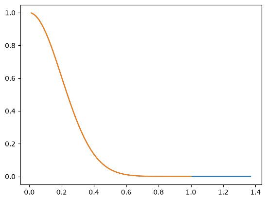
Here is an example of using the DVR basis to interpolate from one radial basis to another. Note that the basis is designed to represent the wavefunction, so we call the interpolation function :meth:~mmfutils.math.bases.CylindricalBasis.Psi

from mmfutils.math.bases import CylindricalBasis
b1 = CylindricalBasis(Nxr=(1, 64), Lxr=(2.0, 1.369))
b2 = CylindricalBasis(Nxr=(1, 64), Lxr=(2.0, 1.0))
x1, r1 = b1.xr
x2, r2 = b2.xr
n1 = np.maximum(0*x1 + (0.25**2 - r1**2), 0)
n1 = 0*x1 + np.exp(-(r1/0.2)**2/2)
n2 = (b1.Psi(np.sqrt(n1), (x2, r2)))**2
plt.clf()
plt.plot(r1.ravel(), n1.ravel())
plt.plot(r2.ravel(), n2.ravel())

[<matplotlib.lines.Line2D at 0x7f3f2649f4d0>]

Transformations

We allow for some transformations of our bases.

Translations

We start with a wavefunction \(\psi(x, t) = f(x-vt)\) that has a constant shape moving to the right at speed \(v\). To simplify the description of this solution, we might want to work with coordinates \(X_v \equiv X = x - vt\) where the wavefunction has the simpler form

\[\begin{gather*} \psi_v(X, t) = f(X) = \psi(x, t) = f(x-vt). \end{gather*}\]

In otherwise, the wavefunction is the same, but the coordinates are different.

This is what we mean by formulating the problem in a frame moving with velocity \(v\) to the right. The moving wave is simpler in such a co-moving frame:

\[\begin{gather*} \psi(x, t) = f(x-vt), \qquad \psi_v(X, t) = f(X). \end{gather*}\]

This transformation is effected by the active translation operator:

\[\begin{gather*} \op{T}_\lambda = \exp\bigl\{\lambda \overbrace{\frac{\op{p}_x}{\I\hbar}}^{-\partial_x}\bigr\}, \qquad \psi(x, t) = \op{T}_{vt}\psi_v(x, t) = \psi_v(x-vt, t), \qquad \psi_v(x, t) = \overbrace{\op{T}_{-vt}}^{\op{T}_{vt}^{-1}}\psi(x, t). \end{gather*}\]

This follows from the expansion of the exponential which generates the Taylor expansion of \(\psi_v(x-vt, t)\) in terms of \(\lambda = vt\).

To derive the equations of motion for the wavefunction \(\psi_v\) in the moving frame, we apply the Hamiltonian:

\[\begin{gather*} \I\hbar \partial_t \psi(x, t) = \op{H}\psi(x, t), \qquad \I\hbar \partial_t \bigl(\op{T}_{vt}\psi_v(x, t)\bigr) = \op{H}\op{T}_{vt}\psi_v(x, t),\\ \I\hbar\dot{\psi}_v(x, t) = \overbrace{\op{T}^{-1}_{vt}\bigl(\op{H}\op{T}_{vt} - \I\hbar\dot{\op{T}}_{vt}\bigr)}^{\op{H}_v}\psi_v(x, t). \end{gather*}\]

Explicitly, for translations, we have \(\I\hbar\dot{\op{T}}_{vt} = v\op{T}_{vt}\op{p}_x\), so:

\[\begin{gather*} \op{H}_{v} = \frac{\op{p}^2}{2m} - v\op{p}_{x} + \overbrace{\op{T}^{-1}_{vt}\op{V}\op{T}_{vt}}^{V(\op{x}+vt)}. \end{gather*}\]

Boosting shifts the dispersion by \(-v\op{p}_x\) and moves the potential. This is a partial Galilean transform. To obtain a full Galilean transformation that restores the form of \(\op{H}\) one needs to include a phase redefinition as discussed on my website.

Rotations

\(\newcommand{\vect}[1]{\vec{#1}}\)One can work analogously with rotations specified by a vector \(\vect{\theta}\) representing a rotation by angle \(\theta = \norm{\vect{\theta}}_2\) about the axis along \(\vect{\theta}\). In cartesian coordinates, the active transformation is effected through the following rotation matrix:

\[\begin{gather*} \mat{R}_\vect{\theta} = e^{\vect{\theta}\times}, \qquad \vect{x} = \mat{R}_\vect{\theta}\vect{X}. \end{gather*}\]

To check our sign, consider rotating about the \(z\) axis so that \(\vect{\theta} = \theta \uvect{z}\). As an active rotation, the rotation matrix should take the point \(\uvect{x} = (1, 0)\) to the point \((\cos\theta, \sin\theta) \approx (1, \theta) = \uvect{x} + \theta\uvect{y}\) for small \(\theta\). Now recall that \(\uvect{x}\times\uvect{y} = \uvect{z}\) and cyclic permutations, so \(\uvect{z}\times\uvect{x} = \uvect{y}\). Hence:

\[\begin{gather*} \mat{R} = \mat{1} + \vect{\theta}\times + \order(\theta^2) \approx \mat{1} + \theta\uvect{z}\times,\qquad \mat{R}\cdot\uvect{x} \approx \uvect{x} + \theta\uvect{z}\times\uvect{x} = \uvect{x} + \theta\uvect{y}. \end{gather*}\]

\(\newcommand{\vect}[1]{\vec{#1}}\)For a rotating frame, one has \(\vect{\theta} = \vect{\omega} t\) which we shall restrict here to \(\vect{\omega} = \omega \uvect{z}\). The equivalent transformation on a wavefunction is:

\[\begin{gather*} \op{R}_{\vect{\theta}} = \exp\Bigl\{\vect{\theta}\cdot\frac{\vect{\op{L}}}{\I\hbar}\Bigr\}, \qquad \psi(\vect{x}, t) = \op{R}_{\omega t}\psi_{\omega t}(\vect{x}, t) = \psi_{\omega t}(\mat{R}_{\omega t}^{-1}\cdot\vect{x}, t). \end{gather*}\]

Explicitly for a rotating frame, \(\I\hbar\dot{\op{R}}_{\vect{\omega} t} = \op{R}_{\vect{\omega} t}\vect{\omega}\cdot\vect{\op{L}}\) so

\[\begin{gather*} \op{H}_{\vect{\omega}} = \frac{\op{p}^2}{2m} - \vect{\omega}\cdot\vect{\op{L}} + \overbrace{\op{R}^{-1}_{\vect{\omega} t}\op{V}\op{R}_{\vect{\omega} t}}^{V(\mat{R}_{\vect{\omega}t}^{-1}\cdot\vect{x})}. \end{gather*}\]

\[\begin{gather*} \op{L}_z = \op{x}\op{p}_y - \op{y}\op{p}_x = \hbar(\op{x}\op{k}_y - \op{y}\op{k}_x), \qquad -\frac{\hbar^2}{2m}\left(\nabla^2 + \frac{2m}{\hbar}\omega_z \bigl(\op{x}(\overbrace{-\I\nabla_y}^{k_y})-\op{y}(\overbrace{-\I\nabla_x}^{k_x})\bigr)\right) \end{gather*}\]

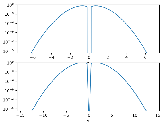
Test

As a simple test, we compute the laplacian in a stationary and a rotating frame:

\[\begin{gather*} f(x, y) = (x+\I y)e^{-x^2-y^2} = re^{-r^2}e^{\I\theta}, \qquad \nabla^2f = \bigl(4(x^2+y^2) - 8\bigr)f, \qquad \frac{\op{L}_z}{\hbar}f = f. \end{gather*}\]

from importlib import reload
from mmfutils.math.bases import bases

reload(bases)
from mmfutils.plot import imcontourf

N = 32 * 2
L = 14.0
eps = np.finfo(float).eps
b = bases.PeriodicBasis(Nxyz=(N, N), Lxyz=(L, L))
x, y = b.xyz
kx, ky = b._pxyz
f = (x + 1j * y) * np.exp(-(x**2) - y**2)
nabla_f = (4 * (x**2 + y**2) - 8) * f
Lz_f = f
ax = plt.subplot(211)
plt.semilogy(x.ravel(), abs(f)[:, N // 2])
ax.set(xlabel="x", ylim=(eps, 1))
ax = plt.subplot(212)
ft = np.fft.fftshift(b.fftn(f))
plt.semilogy(np.fft.fftshift(kx), (abs(ft) / abs(ft).max())[:, N // 2])
ax.set(xlabel="y", ylim=(eps, 1))

assert np.allclose(nabla_f, b.laplacian(f))
assert np.allclose(Lz_f, b.apply_Lz_hbar(f))
m = 1.1
hbar = 2.2
wz = 3.3
kwz2 = m * wz / hbar
factor = -(hbar**2) / 2 / m
assert np.allclose(
    factor * nabla_f - wz * hbar * Lz_f, b.laplacian(f, factor=factor, kwz2=kwz2)
)

np.allclose(b.laplacian(f, factor=factor, kwz2=kwz2) / b.laplacian(f), factor)

False

plt.plot(
    x.ravel(),
    ((factor * nabla_f - b.laplacian(f, factor=factor, kwz2=-1)) / Lz_f)[:, N // 2],
)
plt.ylim(-3, 3)

/tmp/ipykernel_4271/2635635764.py:3: RuntimeWarning: divide by zero encountered in divide
  ((factor * nabla_f - b.laplacian(f, factor=factor, kwz2=-1)) / Lz_f)[:, N // 2],
/home/docs/checkouts/readthedocs.org/user_builds/gpe/conda/latest/lib/python3.14/site-packages/matplotlib/cbook.py:1719: ComplexWarning: Casting complex values to real discards the imaginary part
  return math.isfinite(val)
/home/docs/checkouts/readthedocs.org/user_builds/gpe/conda/latest/lib/python3.14/site-packages/matplotlib/cbook.py:1355: ComplexWarning: Casting complex values to real discards the imaginary part
  return np.asarray(x, float)

(-3.0, 3.0)