Viscosity Notes 2#
These are some supporting notes for the document Effective Viscosity.
Time Evolution#
Here we consider the time-evolution of the system in terms of the following PDEs:
We start by implementing them as follows, in terms of the density and velocity \(y = (n, u)\):
We start with this simple formulation, and use a finite difference scheme for computing the spatial derivatives with boundary conditions imposed by adding ghost points, extending the arrays so we can use simple finite-difference operators.
How to compute derivatives.
There are ambiguities about how to compute the derivatives when implementing these equations owing to the fact that the Leibniz identity (product rule) is not satisfied by numerical derivative techniques:
Errors/differences introduced this way should vanish in the limit of UV convergence as we take the lattice spacing to zero, but is there a preferred approach? There may be other factors to guide the choice.
Stability: As we shall see, probably the most important criteria is that the evolution be stable in the sense that we do not want any growth of unphysical modes (typically high-frequency modes). This will be a dominant criterion.
Consistency: If the equations follow from a minimization principle or stationary action, then it can be worthwhile ensuring that the equations of motion are a numerically exact implementation of the variation. For example, if one has an action with a spatially dependent effective mass in the Schrödinger equation:
\[\begin{gather*} \mathcal{L} = \frac{\hbar^2}{2m(x)} \abs{\op{D}\psi(x)}^2, \end{gather*}\]then one should implement the Hamiltonian as
\[\begin{gather*} \op{H}\psi = +\op{D}^T\left(\frac{\hbar^2 \op{D}\psi}{2m(x)}\right). \end{gather*}\]Depending on how the numerical derivative \(\mat{D}\) is implemented, one might have \(\op{D}^T = - \op{D}\), yielding the more familiar form from integrating by parts, but this should be explicitly verified.
Conservation: Adherence to the form of conservation laws might suggest computing \(j_{,x}\) above rather than \(n_{,x}u + nu_{,x}\). Good numerical approaches will often ensure that conserved quantities are conserved to numerical accuracy. Note that this can be misleading: solutions may now look nice (as opposed to blowing up) but may be quantitatively inaccurate. It can be valuable to have a technique that does not manifestly conserve particle number, energy, etc. and then to use these to test check the accuracy of the evolution.
Alternatively, if computing the derivative is costly, performance considerations might favour the alternative approach if \(n_{,x}\) and \(u_{,x}\) are needed elsewhere. Remember: don’t make such a decision without actually profiling the performance.
Boundary conditions might also play a role. In our case, we want to fix the current \(j = nu\) flowing into the system, allowing the state to relax (due to the viscosity) to a state with fixed \(j\). This would be quite difficult to implement using ghost points if we were strict about using only \(n\) and \(u\).
We will explore some of these effects below.
Burgers’ Equation#
We start with a simplified version of these equations that admits an analytic solution for testing: Burgers’ equation:
Our system reduces to this in the limit \(\mathcal{P}(x) = 0\) (i.e. \(V(x) = \mathcal{E}(n) = 0\)) with Lamé viscosity \(\nu(n) = \nu n\) with \([\nu] = D^2/T\) in the low density limit \(n(x) \rightarrow 0\). In this case, we have a single equation for the velocity \(u(x)\).
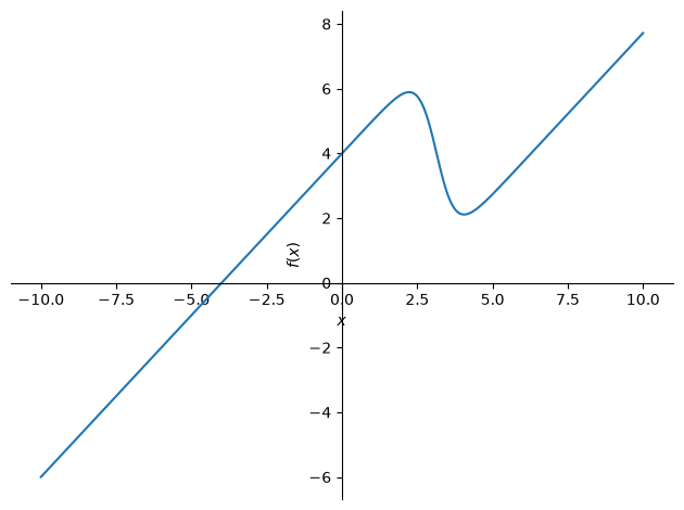
This equation is solvable (see below). Some nice solutions for testing are:
This is a traveling wave with constant shape, but requires Dirichlet boundary conditions far from the transition, or open boundary conditions.
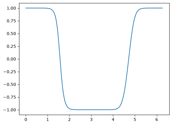
In “Step 4: Burgers’ Equation” of Lorena Barba’s “12 steps to Navier-Stokes”, they present the following approximate, but highly accurate (for small \(\nu\)) periodic solution:
which gives an (almost) periodic velocity profile.
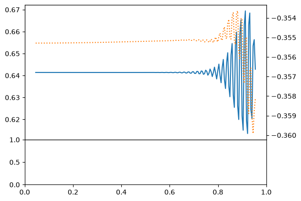
On the Periodicity.
This solution is not periodic (see the margin), but, for small \(\nu\), it is very close. The discontinuity at the boundary,
becomes exponentially small as \(\nu\) gets smaller. I.e., with \(\nu = 0.07\) as used in step 4, the discontinuity is \(\delta u \sim 10^{-61}\).
Solve with the Cole-Hopf Transformation: \(u=-2\nu (\ln \phi)_{,x}\).
Burgers’ equation can be linearized by the Cole-Hopf Transformation:
This is solved by transforming \(\phi \rightarrow \phi e^{f(t)}\), which does not affect \(u(x, t)\) (Why?), to find the heat equation
We now have a linear problem that can be completely solved (do it!):
To get the stated solution, note that, if we start with a Gaussian, it remains a Gaussian:
Recalling that multiplying \(\phi(x, t)\) by a constant function of time does not affect the solution, we can simplify this by dropping the overall factor:
This is a stationary gaussian that expands with time (as per the diffusion equation). To obtain moving solutions, we can simply boost to a moving frame \(u(x, t) \rightarrow u(x-ct, t) + c\). (Remember, \(u\) is a velocity, so we need to add \(c\).) Formally, if \(u(x,t)\) solves Burgers’ equation, then so does
This allows us to express moving and translated solutions in terms of stationary solutions.
Finally, since the equation for \(\phi\) is linear, we can simply add solutions. The stated solution is such a sum with \(c=4\), \(\sigma^2 = 4\nu\), and \(x_0 \in \{0, 2\pi\}\) (in appropriate units):
Solution
The solution is simple in Fourier space. Note that this has exactly the same structure as the Schödinger equation, up to factors of \(\I\) and \(\hbar\):
so we can express our answer in terms of plane-waves (momentum eigenstates)
The state at time \(t\) can simply be expressed in terms of an initial state, and then formulae obtained by inserting the identity:
Converting to position space, we have
The propagator (Green’s function) can thus be computed by completing the square of the Gaussian integral with \(2\nu k_0 t = \I x\), or \(k_0^2 = -x^2/4\nu^2\) with the substitution \(\tilde{k}^2 =\nu(k-k_0)^2 t\) so that \(\d{\tilde{k}} = \sqrt{\nu t} \d{k}\):
Exercise #1: Numerically Solve Burger’s Equation#
Nx = 256
Lx = 2*np.pi
dx = Lx / Nx
x = np.arange(Nx) * dx

# Forward differencing
Df = (np.diag(np.ones(Nx-1), 1) - np.diag(np.ones(Nx), 0))/dx
Df[-1, 0] = 1/dx

# Backwards differencing
Db = (np.diag(np.ones(Nx), 0) - np.diag(np.ones(Nx-1), -1))/dx
Db[0, -1] = -1/dx

assert np.allclose(Df.T, -Db)

# Center difference
Dc = (Df + Db)/2

# Second derivative
D2 = -Df.T @ Df

# Check:
f = np.sin(x)
df = np.cos(x)
ddf = -np.sin(x)

# What error do we expect?  Df and Db should

# Tolerance factor for errors.  Since f, df, etc. all have magnitude
# <= 1, we should be fine with a value of 1 here, but in other cases,
# you may need something up to the magnitude of the appropriate derivatives.
tol_factor = 1.1
assert np.allclose(df, Df @ f, atol=tol_factor * (dx/2), rtol=0)
assert np.allclose(df, Db @ f, atol=tol_factor * (dx/2), rtol=0)
assert np.allclose(df, Dc @ f, atol=tol_factor * (dx**2/6), rtol=0)
assert np.allclose(ddf, D2 @ f, atol=tol_factor * (dx**2/12), rtol=0)

# To test the error formula, these should be tight!
tol_factor = 0.9
assert not np.allclose(df, Df @ f, atol=tol_factor * (dx/2), rtol=0)
assert not np.allclose(df, Db @ f, atol=tol_factor * (dx/2), rtol=0)
assert not np.allclose(df, Dc @ f, atol=tol_factor * (dx**2/6), rtol=0)
assert not np.allclose(ddf, D2 @ f, atol=tol_factor * (dx**2/12), rtol=0)
Notes about the Solution.
First we consider the finite difference errors. For large step sizes, these derive from the Taylor expansion (so-called truncation errors, as opposed to round-off errors that occur at small \(h \lesssim \sqrt{\varepsilon}\)):
(It is not obvious, but one can use the mean-value theorem to show that these error bounds are exact for some point \(\xi \in [x-h, x+h]\). Need Checking.)
nu = 0.1
c = 1.0

def compute_du_dt(u):
    return nu * D2 @ u - u*Df@u

x0 = Lx/4
x1 = 3*Lx/4
c0 = 1
d0 = -1
c1 = 0
d1 = 1
u0 = c0 - d0 * np.tanh(d0*(x-x0)/2/nu)
u1 = c1 + d1 * np.tanh(d1*(x-x1)/2/nu)
u = u0 + u1

from gpe.contexts import FPS

Nt = 100
dt = dx * nu * 0.1
ts = np.arange(Nt) * dt
fig, ax = plt.subplots()

u = u0 + u1
for t in FPS(ts, fig=fig, display=True):
    u += compute_du_dt(u) * dt
    ax.cla()
    ax.plot(x, u)
About the code.
We include here as simple an implementation as possible without any bells and whistles, but have an accompanying code that will be feature-rich. I do this for several reasons:
The documentation stands complete as a reference – no need to refer to another file.
Simple code is easier to understand, and the features can distract from the main point.
Simple code is easy to modify to explore effects like the choice of discretization discussed above: adding flags for all of these features would greatly bloat the production code. Once we learn what is important, we can add only the important features.
Writing simple code like this helps keep me comfortable with rapid prototyping. I find it empowering and reassuring to quickly test things out and often get distracted myself when writing feature-rich code.
Independently implementing code in different ways provides independent checks, helping me find mistakes.
Trying write simple, short, code like this often helps me improve my design.
Note: I actually work as follows:
Start with a simple version that gets me something, often develop in the markdown file, or sometimes switching to a notebook.
Once I have something working, I code this in a module that I can import to play with. I generally prefer to code in a proper Python file with an editor that supports completion, linting, etc. so I don’t make mistakes. Also, once I have importable code, I can easily explore changes without having to copy or re-execute cells in a notebook. Notebooks are good for demonstrating things, but not for extended code.
I then re-write the simple versions for demonstration purposes here in the markdown file, co-developing and improving the pure Python versions as I have ideas.
I highly recommend that you do this too!
import numpy as np


class Flow:
    """Simple class for solving viscous flow problems without a potential."""

    m = 1.2
    g = 1.3
    nu = 0.1  # Viscosity (Lame with power alpha = 1)

    # Lattice
    x0 = -1.0
    x1 = 1.0
    Nx = 200

    # Boundary conditions on the left and right.  None means Neumann.
    n0 = v0 = None  # Left
    n1 = v1 = None  # Right

    def __init__(self, **kw):
        for key in kw:
            if not hasattr(self, key):
                raise ValueError(f"Unknown {key=}")
            setattr(self, key, kw[key])
        self.init()

    def init(self):
        x = np.linspace(self.x0, self.x1, self.Nx + 2)
        self.x = x[1:-1]
        dx = np.diff(x).mean()

        def one(k):
            """Return a diagonal matrix with 1s on the kth diagonal."""
            return np.diag(np.ones(self.Nx + 2 - abs(k)), k=k)

        self._Dx = (one(1) - one(-1)) / 2 / dx
        self._D2x = (one(1) - 2*one(0) + one(-1)) / dx**2

    def get_Eint(self, n, d=0):
        """Equation of state (GPE here)."""
        if d == 0:
            return self.g * n**2 / 2
        elif d == 1:
            return self.g * n
        elif d == 2:
            return self.g
        else:
            return 0

    def get_Vext(self, x, t, d=0):
        """Return the external potential."""
        return 0.0

    def get_nu(self, n, d=0):
        if d == 0:
            return self.nu * n
        else:
            return self.nu

    ######################################################################
    # Dynamics solver
    def apply_D(self, f, f0=None, f1=None, d=1):
        """Return the dth derivative of f."""
        # Pad with external points (Neumann boundary condistions)
        f_ = np.concatenate([f[:1], f, f[-1:]])

        # If values are provided, use these instead
        if f0 is not None:
            f_[0] = f0
        if f1 is not None:
            f_[-1] = f1

        if d == 1:
            D = self._Dx
        elif d == 2:
            D = self._D2x
        return (D @ f_)[1:-1]

    def pack(self, n, u):
        return np.ravel([n, u])

    def unpack(self, y):
        return np.reshape(y, (2, len(y) // 2))

    def compute_dy_dt(self, t, y):
        x = self.x
        n, u = self.unpack(y)
        j = n * u

        n0, v0, n1, v1 = self.n0, self.v0, self.n1, self.v1
        j0 = j1 = None
        if n0 is not None and v0 is not None:
            j0 = n0 * v0
        if n1 is not None and v0 is not None:
            j1 = n1 * v1

        # Compute derivatives
        j_x = self.apply_D(j, j0, j1)
        u_x = self.apply_D(u, v0, v1)
        u_xx = self.apply_D(u, v0, v1, d=2)
        n_x = self.apply_D(n, n0, n1)
        n_xx = self.apply_D(n, n0, n1, d=2)

        dn_dt = -j_x
        du_dt = (
            -u * u_x
            - (self.get_Vext(x, t, d=1) + self.get_Eint(n, d=2) * n_x) / self.m
            # + self.apply_D((self.get_nu(n) * u_x)) / n
            + (self.get_nu(n, d=1) * n_x * u_x + self.get_nu(n) * u_xx) / n
        )
        return self.pack(dn_dt, du_dt)


class FlowStep(Flow):
    """Add a step potential."""
    V_dV = 0.1  # Potential change from right to left.

    def get_Vext(self, x, t, d=0):
        """Return the external potential."""
        if d == 0:
            return np.where(x<0, 0, self.V_dV)
        elif d == 1:
            ind = np.argmin(abs(x-0))
            dx = np.diff(x).mean()
            dV = np.zeros_like(x)
            dV[ind] = self.V_dV / (x[ind+1] - x[ind])
            return dV
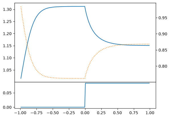
Dam Breaking#
Let’s see how well this works. We start with a dam-breaking problem.
from scipy.integrate import solve_ivp

f = Flow(x0=-1.0, x1=1.0, Nx=200)
x = f.x

n0 = np.where(x < 0, 1.0, 0.5)
v0 = 0*n0
y0 = f.pack(n0, v0)

t_span = (0, 100.0)

res = solve_ivp(f.compute_dy_dt, y0=y0, t_span=t_span, method="BDF")
if not res.success:
    print(res.message)

# Unpack solution
x, ts = f.x, res.t
V = f.get_Vext(x, t=0)
ns, us = res.y.reshape((2, len(x), len(ts)))
fig, axs = plt.subplots(2, 1, height_ratios=(3, 1),
                        gridspec_kw=dict(hspace=0))
ax0, axV = axs
ax1 = ax0.twinx()
ax0.plot(x, ns[:, -1])
ax1.plot(x, us[:, -1], 'C1:')
axV.plot(x, V)
---------------------------------------------------------------------------
ValueError                                Traceback (most recent call last)
Cell In[7], line 26
     22 ax0, axV = axs
     23 ax1 = ax0.twinx()
     24 ax0.plot(x, ns[:, -1])
     25 ax1.plot(x, us[:, -1], 'C1:')
---> 26 axV.plot(x, V)

File ~/checkouts/readthedocs.org/user_builds/gpe/conda/latest/lib/python3.14/site-packages/matplotlib/axes/_axes.py:1792, in Axes.plot(self, scalex, scaley, data, *args, **kwargs)
   1549 """
   1550 Plot y versus x as lines and/or markers.
   1551
   (...)   1789 (``'green'``) or hex strings (``'#008000'``).
   1790 """
   1791 kwargs = cbook.normalize_kwargs(kwargs, mlines.Line2D)
-> 1792 lines = [*self._get_lines(self, *args, data=data, **kwargs)]
   1793 for line in lines:
   1794     self.add_line(line)

File ~/checkouts/readthedocs.org/user_builds/gpe/conda/latest/lib/python3.14/site-packages/matplotlib/axes/_base.py:331, in _process_plot_var_args.__call__(self, axes, data, return_kwargs, *args, **kwargs)
    329     this += args[0],
    330     args = args[1:]
--> 331 yield from self._plot_args(
    332     axes, this, kwargs, ambiguous_fmt_datakey=ambiguous_fmt_datakey,
    333     return_kwargs=return_kwargs
    334 )

File ~/checkouts/readthedocs.org/user_builds/gpe/conda/latest/lib/python3.14/site-packages/matplotlib/axes/_base.py:509, in _process_plot_var_args._plot_args(self, axes, tup, kwargs, return_kwargs, ambiguous_fmt_datakey)
    506     axes.yaxis.update_units(y)
    508 if x.shape[0] != y.shape[0]:
--> 509     raise ValueError(f"x and y must have same first dimension, but "
    510                      f"have shapes {x.shape} and {y.shape}")
    511 if x.ndim > 2 or y.ndim > 2:
    512     raise ValueError(f"x and y can be no greater than 2D, but have "
    513                      f"shapes {x.shape} and {y.shape}")

ValueError: x and y must have same first dimension, but have shapes (200,) and (1,)
from scipy.integrate import solve_ivp

j0 = 1.0
n0 = 1.0
v0 = j0/n0

f = FlowStep(x0=-1.0, x1=1.0, Nx=200, n0=n0, v0=v0)

m_scale = f.m
n_scale = n0
x_scale = 1/n0
v_scale = abs(v0)
E_scale = f.m * v_scale**2

one = np.ones_like(f.x)
y0 = f.pack(n=n0*one, u=v0*one)

t_span = (0, 100.0)

# The default https://github.com/scipy/scipy/issues/18039
res = solve_ivp(f.compute_dy_dt, y0=y0, t_span=t_span, method="BDF")
if not res.success:
    print(res.message)

# Unpack solution
x, ts = f.x, res.t
V = f.get_Vext(x, t=0)
ns, us = res.y.reshape((2, len(x), len(ts)))
fig, axs = plt.subplots(2, 1, height_ratios=(3, 1),
                        gridspec_kw=dict(hspace=0))
ax0, axV = axs
ax1 = ax0.twinx()
ax0.plot(x/x_scale, ns[:, -1]/n_scale)
ax1.plot(x/x_scale, us[:, -1]/v_scale, 'C1:')
axV.plot(x/x_scale, V/E_scale)
[<matplotlib.lines.Line2D at 0x7956a007e900>]
# Here we use a custom `animate` function defined at the start of this file.
# This requires the following coroutine
def draw_frame(f=f, res=res):
    # First initialize the figure and any other computations
    fig, axs = plt.subplots(2, 1, figsize=(4, 3),
                            height_ratios=(3, 1),
                            gridspec_kw=dict(hspace=0))
    ax0, axV = axs
    ax1 = ax0.twinx()

    m_scale = f.m
    n_scale = f.n0
    x_scale = 1/f.n0
    v_scale = abs(f.v0)
    E_scale = f.m * v_scale**2
    t_scale = 1 / (n_scale * v_scale)

    x, ts = f.x, res.t
    ns, us = res.y.reshape((2, len(x), len(ts)))

    x_ = x / x_scale
    ns_ = ns.T / n_scale
    us_ = us.T / v_scale
    ts_ = ts / t_scale

    # Since we will be updating the data, we must scale ylims at the start.
    ax0.set(xlabel="$x$ [$1/n_0$]",
            ylabel="$n$ [$n_0$]",
            ylim=(0, ns_.max()))
    ax1.set(ylabel="$u$ [$v_0$]", ylim=(us_.min(), us_.max()))
    axV.set(ylabel="$V$ [$mv_0^2$]")

    # We first return the figure as the artists first.
    artists = fig

    while True:
        # REQUIRED: The first time through, you must yield the figure `fig`.  After
        # this, if `blit==True`, then you must yield a list of the artists.
        # The results yielded by `get_data` will be passed in here, so `data` must
        # recieve these properly.
        frame = yield artists

        # Now compute the things to plot.
        n_ = ns_[frame]
        u_ = us_[frame]
        V_ = f.get_Vext(x, t=ts[frame])/E_scale
        t_ = ts_[frame]
        title = f"$t={t_:.2f}$ [$1/j_0$]"

        if artists is fig:
            # First time through, plot the data and save the artists
            line_n, = ax0.plot(x_, n_)
            line_u, = ax1.plot(x_, u_, 'C1:')
            line_V, = axV.plot(x_, V_)
            text_title = ax0.set_title(title)
            artists = [line_n, line_u, line_V, text_title]
            continue

        # Every other time, update these
        line_n.set_data(x_, n_)
        line_u.set_data(x_, u_)
        line_V.set_data(x_, V_)
        text_title.set_text(title)


%time anim = animate(draw_frame, len(res.t), interval=10, repeat=False, close=False)
CPU times: user 6 μs, sys: 0 ns, total: 6 μs
Wall time: 10 μs
---------------------------------------------------------------------------
NameError                                 Traceback (most recent call last)
Cell In[9], line 66
     62         line_V.set_data(x_, V_)
     63         text_title.set_text(title)
     64
     65
---> 66 get_ipython().run_line_magic('time', 'anim = animate(draw_frame, len(res.t), interval=10, repeat=False, close=False)')

File <timed exec>:1
----> 1 'Could not get source, probably due dynamically evaluated source code.'

NameError: name 'animate' is not defined
Note
There are two options for viewing these in an HTML document: as an html5 video, or as a JS video. The latter is larger and slowe, so we use the former with some modifications for the width:
If you want to do this for all animations, you can set the following parameter.
#plt.rcParams["animation.html"] = "jshtml"
plt.rcParams["animation.html"] = "html5"
display(anim)
---------------------------------------------------------------------------
NameError                                 Traceback (most recent call last)
Cell In[10], line 3
      1 #plt.rcParams["animation.html"] = "jshtml"
      2 plt.rcParams["animation.html"] = "html5"
----> 3 display(anim)

NameError: name 'anim' is not defined
Another Approach#
An alternative implementation replaces the velocity with the current \(j=nu\):
This is implemented as