import warnings
warnings.filterwarnings("ignore", 
                        category=UserWarning, 
                        message="Numpy fft .* faster than pyfftw.*") 

Getting Started in Higher Dimensions

In Getting Started with the GPE, we looked at Josephson oscillations in 1D trapped gas. (We assume you have read this document.) Here we consider a similar problem, but extended to 3D.

This problem follows the experimental procedure of [Yefsah et al., 2013] where they used a similar procedure to imprint a soliton in the unitary Fermi gas (UFG). They observed that the soliton moved much more slowly, calling it a “heavy soliton. We showed [Bulgac et al., 2014] that, in a symmetric 3D trap, such an imprinted soliton would rapidly decay into a vortex ring, explaining the slow motion. Subsequent experiments [Ku et al., 2014] confirmed that the “heavy soliton” was a “solitonic vortex”, and made clear that the tube as horizontally aligned, causing gravity to break the axial symmetry. We confirmed that, relaxing this symmetry, the vortex rings quickly decay into the observed solitonic vortices [Wlazłowski et al., 2015]. Additional structures were explored experimentally in [Ku et al., 2015] and theoretically in [Wlazłowski et al., 2018].

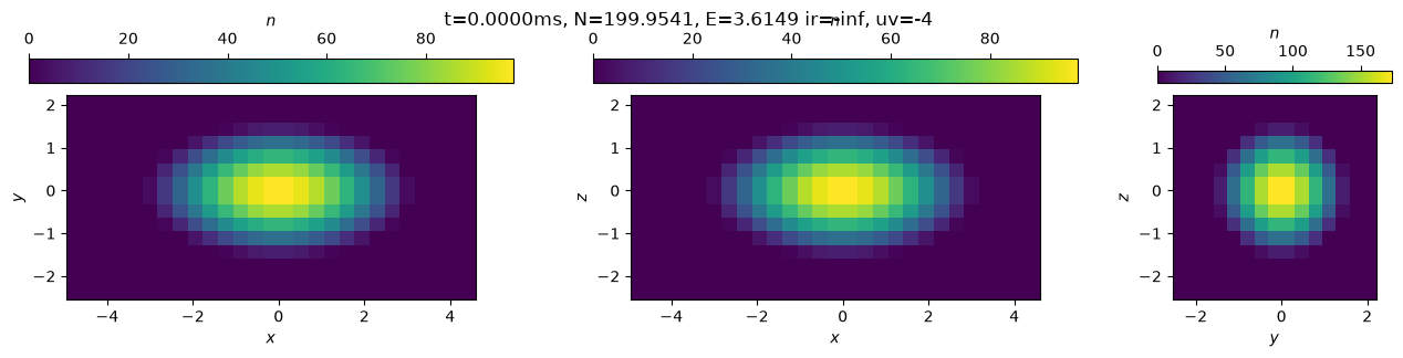
The Problem

The problem we will consider here is the evolution of a dark soliton imprinted in a harmonically trapped gas at some position \(x_s\). We expect the soliton to oscillate back and forth with the trapping period \(T_x\).

We consider a harmonically trapped gas with trapping frequencies \(\omega_x \ll \omega_y, \omega_z\), typically expressed \(\omega = 2\pi f\) where \(f\) is in Hz. The experiments typically report the total number of atoms \(N\), which is related to the chemical potential \(\mu\), and the Thomas-Fermi “radius” \(x_{TF}\) where density vanishes:

\[\begin{gather*} N \approx \frac{4\pi m}{15 g\omega_x\omega_y\omega_z}\left(\frac{2\mu}{m}\right)^{5/2}, \qquad x_{TF} = \frac{1}{\omega_x}\sqrt{\frac{2\mu}{m}}. \end{gather*}\]

Do it! Derive this using the Thomas-Fermi approximation.

The Thomas-Fermi (TF) approximation neglects the gradient terms, assuming that the equation of state matches the potential locally:

\[\begin{gather*} \mu \approx \overbrace{V(\vect{r})}^{\mathclap{\frac{m}{2}(\omega_x^2x^2 + \omega_y^2y^2 + \omega_z^2z^2)}} + \underbrace{\mathcal{E}'\bigl(n(\vect{r})\bigr)}_{\mathcal{E}'_{GPE}(n)=gn}. \end{gather*}\]

Inverting this, we have the Thomas-Fermi approximation

\[\begin{gather*} n_{TF}(\vect{r}) = \begin{cases} \frac{\mu - V(\vect{r})}{g} & \text{where} \quad \mu \geq V(\vect{r}), \\ 0 & \text{otherwise}. \end{cases} \end{gather*}\]

We can directly integrate, but to make the integration variable spherically symmetric, it is useful to introduce the variables \(q_i = \omega_i r_i\) so that the integral becomes

\[\begin{align*} N &= \int n(\vect{r})\d^3{r} = \frac{1}{\omega_x\omega_y\omega_z}\int n(q)\d^3{q}\\ &= \frac{1}{g\omega_x\omega_y\omega_z}\int_0^{\overbrace{\sqrt{2\mu/m}}^{Q}}4\pi q^2\d{q}\; \left(\mu - \frac{m q^2}{2}\right)\\ &= \frac{4\pi}{g\omega_x\omega_y\omega_z} \left(\frac{\overbrace{\mu}^{mQ^2/2} Q^3}{3} - \frac{m Q^5}{10}\right) = \frac{4\pi}{g\omega_x\omega_y\omega_z}\frac{m Q^5}{15} \end{align*}\]

As a quick check, the dimensions are correct and \(N\) is dimensionless as expected (note: \([\mu] = [gn] = E = MD^2/T^2\), \([g] = MD^5/T^2\)):

\[\begin{gather*} [N] = \frac{1}{\frac{MD^5}{T^2}\frac{1}{T^3}}M\frac{D^5}{T^5} = 1. \end{gather*}\]

The TF radius along an appropriate axis is where \(\mu = m\omega_x^2x^2/2\) so the density vanishes.

As a check, consider Eq. (6.34) from [Pethick and Smith, 2002]:

\[\begin{gather*} N = \frac{8\pi}{15}\left(\frac{2\mu}{m\bar{\omega}^2}\right)^{3/2}\frac{\mu}{U_0} = \frac{4\pi m}{15 g \bar{\omega}^3}\left(\frac{2\mu}{m}\right)^{5/2} \tag{6.34} \end{gather*}\]

where \(U_0 = g\), and \(\bar{\omega} = \sqrt[3]{\omega_x\omega_y\omega_z}\) is the geometric mean of the frequencies.

Check the documentation for StateWithExperimentMixin to see which functions are needed in your Experiment class to satisfy the IExperiment interface. Many of these can be defined by simply inheriting from e.g. GPEMixin and HOMixin. E.g.:

• get_Vext(): Defines the external potential. We get this from HOMixin which defines a harmonic trap from the frequencies get_ws(), get_ws()

We introduce here a slightly more general way of dealing with states. Instead of putting everything into the State class, we create an Experiment class and pass this to the state. We inform our state by inheriting from StateWithExperimentMixin which delegates the appropriate functions to the experiment. This allows us to use a variety of different states that all use the same Experiment, e.g., to use different states for different 3D approximations:

• gpe.tube: Effective 1D Non-Polynomial Schrödinger Equation (NPSEQ) and Dynamically Rescaled GPE (dr-GPE) that approximates simple radial dynamics. Does not allows vortex rings etc.

• gpe.axial: Effective 2D assuming axial (rotational) symmetry.

• gpe.bec: Full 3D simulations.

We start with the formulation in 3D, then specialize.

import numpy as np
import matplotlib.pyplot as plt

import gpe.bec, gpe.utils, gpe.minimize

u = gpe.bec.u

class StateMixin(gpe.utils.StateWithExperimentMixin):
    def get_ws(self, t=None):
        # Needed for codes that support expansion.
        return self.experiment.ws


class State(StateMixin, gpe.bec.StateBase):
    """Simple 3D state."""
    pass


class Experiment(gpe.bec.GPEMixin, gpe.bec.HOMixin, gpe.utils.ExperimentBase):
    """Experiment for domain wall oscillations."""
    # Physical parameters for experiemnt
    trapping_frequencies_Hz = (50.0, 100.0, 100.0)  # Trap frequencies
    Ntot = 200       # Number of particles
    m = u.m_Rb87     # We use 87Rb here.
    hbar = u.hbar    # Physical units according to `gpe.bec.u`.
    species = (2,0)  # Which hyperfine state - defines the interaction.
    
    # Numerical parameters
    L_TF = 1.5               # Length of box as a fraction of the TF radius
    dx_healing_length = 0.5  # Minimum resolution
    
    # Parameter for knife-edge and phase imprint
    x0_TF = 0.1                 # Location of imprint in units of x_TF
    V0_mu = 2.0                 # Depth of the knife
    sigma_healing_length = 0.2  # With of knife in healing_lengths
    dphi = np.pi                # Initial phase difference
    
    State = State               # Which state to use
    
    def init(self):
        """Perform any initializations."""
        a = u.scattering_lengths[(self.species, self.species)]
        self.g = 4*np.pi * self.hbar**2 * a / self.m
        
        self.ws = 2*np.pi * np.asarray(self.trapping_frequencies_Hz) * u.Hz
        
        # We use the trap frequency as a time unit.
        self.t_unit = 2*np.pi / self.ws[0]
        self.t_label = "$T_x$"
        
        # Use TF results to get mu from Ntot
        V_TF = self.m/2 * (
            15*self.g * np.prod(self.ws) * self.Ntot
            / (4*np.pi * self.m))**(2/5)
            
        self.mu = V_TF  # Not accurate
        self.healing_length = self.hbar / np.sqrt(2 * self.m * self.mu)
        rs_TF = np.sqrt(2 * self.mu / self.m) / self.ws
        self.Lxyz = 2 * self.L_TF * rs_TF
        dx = self.dx_healing_length * self.healing_length
        
        # Get good lattice sizes for use with the FFT (small prime factors)
        self.Nxyz = list(map(gpe.utils.get_good_N, self.Lxyz / dx))
        
        self.V0 = self.V0_mu * self.mu
        self.sigma = self.sigma_healing_length * self.healing_length
        
        x_TF = rs_TF[0]
        self.x0 = self.x0_TF * x_TF
        
        self.state_args = dict(
            Nxyz=self.Nxyz, Lxyz=self.Lxyz, 
            mu=self.mu, g=self.g, m=self.m, hbar=self.hbar)
        
        super().init()  # Be sure to call other init() functions.
        
    def get_state(self):
        """Return (quickly) a state instance."""
        return self.State(experiment=self, **self.state_args)

    def get_initial_state(self):
        """Return the initial state for a simulation."""
        state0 = self.get_state()
        
        # The experiments imprint the phase with an external step potential.
        # We cheat here by minimizing with the desired phase.
        x = state0.xyz[0] + np.zeros(state0.shape)  # Sometimes we need a full array
        phase = np.exp(1j*np.where(x < self.x0, -self.dphi/2, self.dphi/2))
        minimizer = gpe.minimize.MinimizeStateFixedPhase(state0, phase=phase, fix_N=True)
        state0 = minimizer.minimize()
        
        # Always use a fresh state in case the minimizer alters cooling_phase etc.
        state = self.get_state()
        state.set_psi(state0.get_psi())
        return state
    
    def get_Vknife(self, x):
        """Return the knife-edge potential which divides the cloud in two."""
        return self.V0 * np.exp(-(x/self.sigma)**2/2)

    @gpe.utils.i_know_this_is_slow  # Suppresses PerformanceWarning
    def get_Vext(self, state):
        """Return Vext. The state will call this."""
        xyz = state.get_xyz()
        Vext = self.m / 2 * sum([(w*x)**2 for w, x in zip(self.ws, xyz)])
        if state.initializing or state.t < 0:
            # This code only gets executed if we are initializing the state, or evolving
            # for negative times (wehich we might do for imaginary time initialization).
            # We initialize with the knife edge in place.  We then evolve without the
            # knife.  Note: The underlying code calls `get_Vext_mu()` which also
            # subtracts `self.mu`: we should not do that here.
            x = xyz[0]
            Vext += self.get_Vknife(x-self.x0)
        return Vext
        
e = Experiment(V0_mu=0)  # Turn off knife to check TF approximation 
print(f"{e.Nxyz = }: states will take {np.prod(e.Nxyz)*16/1024**2:.2g}MiB")
s0 = e.get_state()
s0.plot()
assert np.allclose(s0.get_N(), e.Ntot, rtol=1e-3)

e.Nxyz = [27, 15, 15]: states will take 0.093MiB

/home/docs/checkouts/readthedocs.org/user_builds/gpe/conda/latest/lib/python3.14/site-packages/gpe/bec.py:1112: RuntimeWarning: divide by zero encountered in log10
  ir, uv = map(np.log10, self.get_convergence())

e = Experiment()
%time s = e.get_initial_state()
s.plot()
print(f"μ/ℏω = {s.mu/(s.hbar*e.ws[1]):.4f}")

CPU times: user 5.3 s, sys: 3.8 ms, total: 5.31 s
Wall time: 2.67 s
μ/ℏω = 1.0865

from pytimeode.evolvers import EvolverABM

def evolve(state, periods=1, Nt=100, dt_t_scale=0.1):
    """Evolve the state for the specified number of periods."""
    e = state.experiment
    T = 2*np.pi * periods / e.ws[0]
    dT = T / Nt
    dt = dt_t_scale * state.t_scale
    steps = int(max([np.ceil(dT / dt), 2]))
    dt = dT / steps

    ev = EvolverABM(state, dt=dt)
    states = [ev.get_y()]

    for frame in range(Nt):
        ev.evolve(steps)
        states.append(ev.get_y())
    
    return states

def plot(states):
    s = states[-1]
    e = s.experiment
    Tx = 2*np.pi / e.ws[0]
    ns = np.array([s.get_density_x() for s in states])
    ts = [s.t for s in states]
    xs = s.xyz[0].ravel()
    fig, ax = plt.subplots()
    mesh = ax.pcolormesh(ts / Tx, xs / u.micron, ns.T * u.micron)
    fig.colorbar(mesh, ax=ax, label="$n_{1D}$ [1/micron]")
    ax.set(xlabel="$t/T_x$", ylabel="$x$ [micron]")

e = Experiment()
%time s = e.get_initial_state()
%time states = evolve(s, periods=2)

CPU times: user 4.97 s, sys: 8.84 ms, total: 4.98 s
Wall time: 2.51 s
CPU times: user 20 s, sys: 1.61 s, total: 21.6 s
Wall time: 11.1 s

Show code cell source

Hide code cell source

def get_rel_max_edges(psi):
    """Return the maximum relative abs values of psi on the box edges."""
    return max([abs(np.rollaxis(psi, n)[(0, -1), ... ]).max()
                for n in range(len(psi.shape))]) / abs(psi).max()

def check_convergence(states):
    """Plot the convergence metrics."""
    ts = np.array([s.t for s in states])
    Es = np.array([s.get_energy() for s in states])
    Ns = np.array([s.get_N() for s in states])
    psi_edges = np.array([get_rel_max_edges(s.get_psi()) for s in states])
    psik_edges = np.array([get_rel_max_edges(np.fft.fftshift(np.fft.fftn(s.get_psi()))) 
                           for s in states])
    fig, axs = plt.subplots(2, 1, figsize=(4, 3), 
                            sharex=True, constrained_layout=True)
    ax = axs[0]
    ax.plot(ts/e.t_unit, Es/Es[0] - 1, label="$E$")
    ax.plot(ts/e.t_unit, Ns/Ns[0] - 1, label="$N$")
    ax.set(ylabel="Rel. change")
    ax.legend()
    ax = axs[1]
    ax.semilogy(ts/e.t_unit, psi_edges, label=r"$x$")
    ax.semilogy(ts/e.t_unit, psik_edges, label=r"$k$")
    ax.set(xlabel=f"$t$ [{e.t_label}]", ylabel=r"Max value on $\partial$.")
    ax.legend()
    return fig

check_convergence(states);

It is always good to check the accuracy of your simulation. In the above code, we check that the energy and particle number are conserved to 9 digit. We also look at the relative magnitude of the wavefunction at the edge of the box in both position and momentum space. In this case, we have okay convergence in momentum space, but the box is too small. From a convergence standpoint this is fine – we have conserved energy etc. But, we are not simulating the physics we think we are – we are really looking at dynamics in a periodic lattice of harmonic traps where the atoms can spill over the walls. Playing a bit, we find L_TF = 2.5 reduces the boundary effects to a similar level.

Warning: When I initially made this tutorial, I accidentally chose too large of a value for dt_t_scale=0.2 in evolve. This led to the evolution seen to the right. The evolution looks like it might be qualitatively valid, but some issues become apparent: note that the final state has occupancy in the corners of the box. The most important check is that the energy was not conserved as demonstrated below (see Issue #22).

Show code cell source

Hide code cell source

def error():
    # Put this in a function so we don't pollute the global namespace
    # i.e. states.
    e = Experiment()
    s = e.get_initial_state()
    states = evolve(s, periods=2, dt_t_scale=0.2)
    plot(states);
    display(plt.gcf())
    plt.close('all')
    fig, ax = plt.subplots(figsize=(4, 1));
    states[-1].plot(axs=[ax]);
    display(plt.gcf())
    plt.close('all')
    check_convergence(states);
error()

WARNING:matplotlib.axes._base:Ignoring fixed y limits to fulfill fixed data aspect with adjustable data limits.
WARNING:matplotlib.axes._base:Ignoring fixed y limits to fulfill fixed data aspect with adjustable data limits.

plot(states);

Notice that the frequency of the soliton is close, but not exactly commensurate with the trapping frequency. This is an indication that the excitation is almost a domain wall, but that that there are additional excitations. Here is the final state:

states[-1].plot();

Axial Symmetry

For these simulations, we have strict axial symmetry. Thus, we should be able to work in cylindrical coordinates. This is done by gpe.axial. We can use the same experiment, but need to use a different state class.

import gpe.axial

# Note: StateMixing must come first so that we can assign the experiment.
class StateAxial(StateMixin, gpe.axial.StateAxialBase):
    pass


class ExperimentAxial(Experiment):
    # This is much cheaper, so we can be more generous.
    L_TF = 2.0
    dx_healing_length = 0.4
    
    State = StateAxial
    def init(self):
        super().init()
        Nxr = (self.Nxyz[0], max(self.Nxyz[1:]) // 2 + 1)
        Lxr = (self.Lxyz[0], max(self.Lxyz[1:]) / 2.0)

        # Current code requies a basis... this should be fixed
        self.state_args['basis'] = gpe.axial.CylindricalBasis(Nxr=Nxr, Lxr=Lxr)
        self.state_args.pop('Nxyz')
        self.state_args.pop('Lxyz')
        
e = ExperimentAxial(V0_mu=0)
s = e.get_state()
assert np.allclose(s.get_N(), e.Ntot, rtol=1e-2)
print(s.shape)
e = ExperimentAxial()
s = e.get_state()
s.plot()

(np.int64(45), np.int64(13))

[<Axes: title={'center': 't= 0ms, N=166.21, E=5.648, lam=1'}, ylabel='n'>]

e_axial = ExperimentAxial()
%time s_axial = e_axial.get_initial_state()
s_axial.plot()

CPU times: user 1.98 s, sys: 1.78 ms, total: 1.98 s
Wall time: 993 ms

[<Axes: title={'center': 't= 0ms, N=166.21, E=1.2496, lam=1'}, ylabel='n'>]

%time states_axial = evolve(s_axial, periods=2)

CPU times: user 34 s, sys: 160 ms, total: 34.2 s
Wall time: 17.2 s

Show code cell source

Hide code cell source

ts = np.array([s.t for s in states_axial])
Es = np.array([s.get_energy() for s in states_axial])
Ns = np.array([s.get_N() for s in states_axial])

fig, ax = plt.subplots(figsize=(4, 1))
ax.plot(ts/e_axial.t_unit, Es/Es[0] - 1, label="$E$")
ax.plot(ts/e_axial.t_unit, Ns/Ns[0] - 1, label="$N$")
ax.set(xlabel=f"$t$ [{e_axial.t_label}]", ylabel="Rel. change")
ax.legend();

plot(states_axial)

Let’s make a movie comparing the two simulations. We can use gpe.contexts.FPS for this.

from mmf_contexts import FPS

fig, ax = plt.subplots()
for s, sa in FPS(list(zip(states, states_axial)), fig=fig, embed=True):
    ax.cla()
    ax.plot(s.x, s.get_density_x())
    ax.plot(sa.x, sa.get_density_x())
    ax.set(xlabel="$x$ [micron]", ylabel="$n_{1D}$ 1/micron")

Tube NPSEQ

An extension of the NPSEQ allows one to deal with time-dependent radial trapping frequencies, including the common case of turning off the trap and letting the cloud expand for imaging. This results in the Dynamically Rescaled GPE (dr-GPE), which is also implemented in the gpe.tube module.

If not too many radial modes are populated, then one might expect that the radial degrees of freedom can be “integrated out”. One way of doing this results in an effective 1D theory called the Non-Polynomial Schrödinger Equation (NPSEQ).

from importlib import reload
import gpe.tube;reload(gpe.tube)

# Note: StateMixing must come first so that we can assign the experiment.
class StateTube(StateMixin, gpe.tube.StateGPEdrZ):
    pass

class ExperimentTube(Experiment):
    # This is much cheaper, so we can be more generous.
    L_TF = 2.0
    dx_healing_length = 0.4
    
    State = StateTube
    
    def init(self):
        super().init()
        Nx = self.Nxyz[0]
        Lx = self.Lxyz[0]
        self.state_args.update(Nxyz=(Nx,), Lxyz=(Lx,))
        state = self.get_state()
        
        
e = ExperimentTube(V0_mu=0)
s = e.get_state()
assert np.allclose(s.get_N(), e.Ntot, rtol=1e-2)
print(s.shape)
e_tube = ExperimentTube()
s_tube = e_tube.get_state()
s_tube.plot()

---------------------------------------------------------------------------
AssertionError                            Traceback (most recent call last)
Cell In[16], line 25
     21 
     22 
     23 e = ExperimentTube(V0_mu=0)
     24 s = e.get_state()
---> 25 assert np.allclose(s.get_N(), e.Ntot, rtol=1e-2)
     26 print(s.shape)
     27 e_tube = ExperimentTube()
     28 s_tube = e_tube.get_state()

AssertionError: 

e_tube = ExperimentTube()
%time s_tube = e_tube.get_initial_state()
s_tube.plot()

CPU times: user 4.34 s, sys: 9.91 ms, total: 4.35 s
Wall time: 2.19 s

[<Axes: >]

%time states_tube = evolve(s_tube, periods=2)

CPU times: user 19.8 s, sys: 110 ms, total: 19.9 s
Wall time: 10 s

Show code cell source

Hide code cell source

ts = np.array([s.t for s in states_tube])
Es = np.array([s.get_energy() for s in states_tube])
Ns = np.array([s.get_N() for s in states_tube])

fig, ax = plt.subplots(figsize=(4, 1))
ax.plot(ts/e_tube.t_unit, Es/Es[0] - 1, label="$E$")
ax.plot(ts/e_tube.t_unit, Ns/Ns[0] - 1, label="$N$")
ax.set(xlabel=f"$t$ [{e_tube.t_label}]", ylabel="Rel. change")
ax.legend();

plot(states_tube)

w_x, w_perp = e.ws[0], e.ws[1]
x_TF = np.sqrt(2*e.mu /e.m)/w_x
m, h = e.m, e.hbar
hw = e.hbar*w_perp
V_TF = -hw
#print(V_TF, s.get_V_TF_from_mu(s.mu))
V = np.linspace(-e.mu, 0, 1000)
mu_eff_hw = (V_TF - V) / hw + 1
sigma2w = h * (mu_eff_hw + np.sqrt(mu_eff_hw**2 + 3.0)) / (3 * m)
n_1D = 2 * np.pi * m * np.maximum(0, sigma2w**2 - (h / m) ** 2) / e.g
plt.plot(V/e.mu, sigma2w)
plt.plot(V/e.mu, n_1D)

#plt.plot(V_ext/e.mu, s.get_n_TF(V_TF=V_TF, V_ext=V_ext))

[<matplotlib.lines.Line2D at 0x77e890d45fd0>]

V_TF = s.get_V_TF_from_mu(s.mu)
plt.plot(s.x, s.get_Vext()/s.mu)
plt.axhline([V_TF/s.mu])
plt.ylim(-1, 0)
s.get_n_TF(V_TF=V_TF)

array([0.        , 0.        , 0.        , 0.        , 0.        ,
       0.        , 0.        , 0.        , 0.        , 0.        ,
       0.        , 0.        , 0.        , 0.        , 0.        ,
       0.        , 0.        , 0.        , 0.        , 0.        ,
       0.44916321, 0.91866913, 1.15342209, 1.15342209, 0.91866913,
       0.44916321, 0.        , 0.        , 0.        , 0.        ,
       0.        , 0.        , 0.        , 0.        , 0.        ,
       0.        , 0.        , 0.        , 0.        , 0.        ,
       0.        , 0.        , 0.        , 0.        , 0.        ])

In principle this should work, but something is askew. One issue that can arise here is that the tube code requires at least one mode to be occupied in the radial direction, which requires \(\mu > \hbar \omega_\perp\), exceeding the radial zero-point energy. To see this, note that the effective potential for the tube code is

\[\begin{gather*} \newcommand{\abs}[1]{\lvert#1\rvert} \newcommand{\I}{\mathrm{i}} \I\hbar \dot{\psi} = \Biggl( \frac{-\hbar^2\nabla_z^2}{2m} + \frac{\hbar^2}{2m\sigma^2} + \frac{m\omega_\perp^2\sigma^2}{2} + \frac{g\abs{\psi}^2}{2\pi\sigma^2} \Biggr)\psi,\\ \frac{m\omega_\perp^2}{2}\sigma^4 = \underbrace{ \frac{\hbar^2}{2m} + \frac{g\abs{\psi}^2}{4\pi} }_{\text{minimize energy}} , \quad \text{or} \quad \frac{m\omega_\perp^2}{2}\sigma^4 = \underbrace{ \frac{\hbar^2}{2m} + \frac{g\abs{\psi}^2}{2\pi} }_{\text{minimize chemical potential}}. \end{gather*}\]

\[ \frac{\hbar^2}{2m\sigma^2} + \frac{m\omega_\perp^2\sigma^2}{2} + \frac{gn_1}{2\pi\sigma^2} = 0 \]

\[\begin{split} V_{TF} + \hbar\omega_\perp - \mu = 0\\ \omega_\perp \sigma^2 \geq \frac{\hbar}{m}, \qquad \mu \geq \hbar\omega_\perp \end{split}\]

s.get_n_TF(V_TF=V_TF)

array([0.        , 0.        , 0.        , 0.        , 0.        ,
       0.        , 0.        , 0.        , 0.        , 0.        ,
       0.        , 0.        , 0.        , 0.        , 0.        ,
       0.        , 0.        , 0.        , 0.        , 0.        ,
       0.44916321, 0.91866913, 1.15342209, 1.15342209, 0.91866913,
       0.44916321, 0.        , 0.        , 0.        , 0.        ,
       0.        , 0.        , 0.        , 0.        , 0.        ,
       0.        , 0.        , 0.        , 0.        , 0.        ,
       0.        , 0.        , 0.        , 0.        , 0.        ])

print(f"μ/ℏω = {s.mu/(s.hbar*s.w0_perp):.4f}")

μ/ℏω = 1.0865

kw = dict(dx_healing_length=0.2, sigma_healing_length=0.1)

e0 = ExperimentAxial(**kw)
s0 = e0.get_state()
plt.plot(s0.xyz[0], s0.get_Vext()[:, 0])

e = ExperimentTube(**kw)
s = e.get_state()
plt.plot(s.xyz[0], s.get_Vext())

[<matplotlib.lines.Line2D at 0x77e890622660>]

e = ExperimentTube(**kw)
%time s = e.get_initial_state()
s.plot()

CPU times: user 2.06 s, sys: 6.89 ms, total: 2.06 s
Wall time: 1.05 s

[<Axes: >]

%time states = evolve(s, periods=2)
plot(states)
plt.figure()
states[-1].plot()

CPU times: user 1min 23s, sys: 478 ms, total: 1min 23s
Wall time: 42 s

[<Axes: >]

Tube TF Issue

import numpy as np
import matplotlib.pyplot as plt

%load_ext autoreload
%autoreload 2

import gpe.bec, gpe.utils, gpe.minimize
import gpe.tube

u = gpe.bec.u

class StateMixin:
    def __init__(self, experiment, **kw):
        self.experiment = experiment
        super().__init__(**kw)
        
    def get_ws(self, t):
        # Needed because the axial code also supports expansion.
        return self.experiment.ws

    def get_Vext(self):
        # Delegate to the experiment.
        return self.experiment.get_Vext(state=self)

# Note: StateMixing must come first so that we can assign the experiment.
class State(StateMixin, gpe.bec.StateBase):
    pass

# Note: StateMixing must come first so that we can assign the experiment.
class StateTube(StateMixin, gpe.tube.StateGPEdrZ):
    pass

class Experiment(gpe.utils.ExperimentBase):
    # Physical parameters for experiemnt
    trapping_frequencies_Hz = (50.0, 200.0, 200.0)  # Trap frequencies
    Ntot = 200       # Number of particles
    m = u.m_Rb87     # We use 87Rb here.
    hbar = u.hbar    # Physical units according to `gpe.bec.u`.
    species = (2,0)  # Which hyperfine state - defines the interaction.
    
    # Numerical parameters
    L_TF = 1.5               # Length of box as a fraction of the TF radius
    dx_healing_length = 0.5  # Minimum resolution
    
    # Parameter for knife-edge and phase imprint
    x0_TF = 0.1         # Location of imprint in units of x_TF
    V0_mu = 2.0         # Depth of the knife
    sigma_micron = 0.1  # With of knife in micron
    dphi = np.pi        # Initial phase difference
    
    State = State       # Which state to use
    
    def init(self):
        """Perform any initializations."""
        a = u.scattering_lengths[(self.species, self.species)]
        self.g = 4*np.pi * self.hbar**2 * a / self.m
        
        self.ws = 2*np.pi * np.asarray(self.trapping_frequencies_Hz) * u.Hz

        # Use TF results to get mu from Ntot
        self.mu = self.m/2 * (
            15*self.g * np.prod(self.ws) * self.Ntot
            / (4*np.pi * self.m))**(2/5)
        
        self.healing_length = self.hbar / np.sqrt(2 * self.m * self.mu)
        rs_TF = np.sqrt(2 * self.mu / self.m) / self.ws
        self.Lxyz = 2 * self.L_TF * rs_TF
        dx = self.dx_healing_length * self.healing_length
        
        # Get good lattice sizes for use with the FFT (small prime factors)
        self.Nxyz = list(map(gpe.utils.get_good_N, self.Lxyz / dx))
        
        self.V0 = self.V0_mu * self.mu
        self.sigma = self.sigma_micron * u.micron
        x_TF = rs_TF[0]
        self.x0 = self.x0_TF * x_TF
        
        self.state_args = dict(
            Nxyz=self.Nxyz, Lxyz=self.Lxyz, 
            mu=self.mu, g=self.g, m=self.m, hbar=self.hbar)
        
        super().init()  # Be sure to call other init() functions.
    
    def get_state(self):
        """Return (quickly) a state instance."""
        return self.State(experiment=self, **self.state_args)

    def get_initial_state(self):
        """Return the initial state for a simulation."""
        state0 = self.get_state()
        
        # The experiments imprint the phase with an external step potential.
        # We cheat here by minimizing with the desired phase.
        x = state0.xyz[0] + np.zeros(state0.shape)  # Sometimes we need a full array
        phase = np.exp(1j*np.where(x < self.x0, -self.dphi/2, self.dphi/2))
        minimizer = gpe.minimize.MinimizeStateFixedPhase(state0, phase=phase, fix_N=True)
        state0 = minimizer.minimize()
        
        # Always use a fresh state in case the minimizer alters cooling_phase etc.
        state = self.get_state()
        state.set_psi(state0.get_psi())
        return state
    
    def get_Vknife(self, x):
        return self.V0 * np.exp(-(x/self.sigma)**2/2)
        
    def get_Vext(self, state):
        """Return Vext. The state will call this."""
        xyz = state.get_xyz()
        Vext = self.m / 2 * sum([(w*x)**2 for w, x in zip(self.ws, xyz)])
        if state.initializing or state.t < 0:
            x = xyz[0]
            Vext -= self.mu + self.get_Vknife(x-self.x0)
        return Vext

class ExperimentTube(Experiment):
    # This is much cheaper, so we can be more generous.
    L_TF = 2.0
    dx_healing_length = 0.4
    
    State = StateTube
    
    def init(self):
        super().init()
        Nx = self.Nxyz[0]
        Lx = self.Lxyz[0]

        # Current code requies a basis... this should be fixed
        self.state_args.update(Nxyz=(Nx,), Lxyz=(Lx,))
        state = self.get_state()
        #self.mu = state.get_mu_from_V_TF(self.mu) #/2.03435
        self.state_args.update(mu=self.mu)
        #self.state_args.update(x_TF=3.0)

e0 = Experiment(V0_mu=0)  # Turn off knife to check TF approximation 
s0 = e0.get_state()
#s0.plot()
assert np.allclose(s0.get_N(), e0.Ntot, rtol=1e-3)

e = ExperimentTube(V0_mu=0)
s = e.get_state()
s.plot()
plt.plot(s0.xyz[0].ravel(), s0.get_density_x(), '--')
assert np.allclose(s.get_N(), e.Ntot, rtol=1e-2)

%connect_info

{
  "shell_port": 37235,
  "iopub_port": 51355,
  "stdin_port": 32951,
  "control_port": 36281,
  "hb_port": 58605,
  "ip": "127.0.0.1",
  "key": "c9da1078-8b4425843abbdb1d5dad68b6",
  "transport": "tcp",
  "signature_scheme": "hmac-sha256",
  "kernel_name": "python3"
}

Paste the above JSON into a file, and connect with:
    $> jupyter <app> --existing <file>
or, if you are local, you can connect with just:
    $> jupyter <app> --existing /tmp/tmptnqpnn85.json
or even just:
    $> jupyter <app> --existing
if this is the most recent Jupyter kernel you have started.

x = s.xyz[0]
V_ext = s.get_Vext()
V_TF = s.get_V_TF(x_TF=3.0)
print(V_TF)
n_TF = s.get_n_TF(V_TF=V_TF)
#plt.plot(x, V_ext)
plt.plot(x, n_TF)
plt.plot(x, n_1D)

0.009570261831528579

---------------------------------------------------------------------------
ValueError                                Traceback (most recent call last)
Cell In[29], line 8
      4 print(V_TF)
      5 n_TF = s.get_n_TF(V_TF=V_TF)
      6 #plt.plot(x, V_ext)
      7 plt.plot(x, n_TF)
----> 8 plt.plot(x, n_1D)

File ~/checkouts/readthedocs.org/user_builds/gpe/conda/latest/lib/python3.14/site-packages/matplotlib/pyplot.py:3838, in plot(scalex, scaley, data, *args, **kwargs)
   3830 @_copy_docstring_and_deprecators(Axes.plot)
   3831 def plot(
   3832     *args: float | ArrayLike | str,
   (...)   3836     **kwargs,
   3837 ) -> list[Line2D]:
-> 3838     return gca().plot(
   3839         *args,
   3840         scalex=scalex,
   3841         scaley=scaley,
   3842         **({"data": data} if data is not None else {}),
   3843         **kwargs,
   3844     )

File ~/checkouts/readthedocs.org/user_builds/gpe/conda/latest/lib/python3.14/site-packages/matplotlib/axes/_axes.py:1777, in Axes.plot(self, scalex, scaley, data, *args, **kwargs)
   1534 """
   1535 Plot y versus x as lines and/or markers.
   1536 
   (...)   1774 (``'green'``) or hex strings (``'#008000'``).
   1775 """
   1776 kwargs = cbook.normalize_kwargs(kwargs, mlines.Line2D)
-> 1777 lines = [*self._get_lines(self, *args, data=data, **kwargs)]
   1778 for line in lines:
   1779     self.add_line(line)

File ~/checkouts/readthedocs.org/user_builds/gpe/conda/latest/lib/python3.14/site-packages/matplotlib/axes/_base.py:297, in _process_plot_var_args.__call__(self, axes, data, return_kwargs, *args, **kwargs)
    295     this += args[0],
    296     args = args[1:]
--> 297 yield from self._plot_args(
    298     axes, this, kwargs, ambiguous_fmt_datakey=ambiguous_fmt_datakey,
    299     return_kwargs=return_kwargs
    300 )

File ~/checkouts/readthedocs.org/user_builds/gpe/conda/latest/lib/python3.14/site-packages/matplotlib/axes/_base.py:494, in _process_plot_var_args._plot_args(self, axes, tup, kwargs, return_kwargs, ambiguous_fmt_datakey)
    491     axes.yaxis.update_units(y)
    493 if x.shape[0] != y.shape[0]:
--> 494     raise ValueError(f"x and y must have same first dimension, but "
    495                      f"have shapes {x.shape} and {y.shape}")
    496 if x.ndim > 2 or y.ndim > 2:
    497     raise ValueError(f"x and y can be no greater than 2D, but have "
    498                      f"shapes {x.shape} and {y.shape}")

ValueError: x and y must have same first dimension, but have shapes (90,) and (1000,)

if False:
        V_TF = s.get_V_TF(x_TF=3.0)
        g = V_ext = None
        self = s
        zero = np.zeros(self.shape)
        if g is None:
            g = self.g
        if V_ext is None:
            V_ext = self.get_Vext()
        V = V_ext + zero

        h = self.hbar
        m = self.m
        w = self.w0_perp
        hw = h * w
        mu_eff_hw = (V_TF - V) / hw
        mu_eff_hw += 1.0  # This is the extra hbar*w0_perp piece
        sigma2w = h * (mu_eff_hw + np.sqrt(mu_eff_hw**2 + 3.0)) / (3 * m)
        n_1D = 2 * np.pi * m * np.maximum(zero, sigma2w**2 - (h / m) ** 2) / g

plt.plot(V)

if False:
        h = self.hbar
        m = self.m
        w = self.w0_perp
        hw = h * w
        mu_eff_hw = (V_TF - V) / hw
        mu_eff_hw += 1.0  # This is the extra hbar*w0_perp piece
        sigma2w = h * (mu_eff_hw + np.sqrt(mu_eff_hw**2 + 3.0)) / (3 * m)
        n_1D = 2 * np.pi * m * np.maximum(zero, sigma2w**2 - (h / m) ** 2) / g

self = s
x_TF = 3.0
V_TF = self.get_V_TF(x_TF=x_TF)
s.get_V_TF_from_mu(self.get_mu_from_V_TF(V_TF=self.get_V_TF(x_TF=x_TF))), V_TF
self.get_mu_from_V_TF(V_TF=self.get_V_TF(x_TF=x_TF)), s.mu
s.get_mu_from_V_TF(self.mu), V_TF