import mmf_setup;mmf_setup.nbinit()
%pylab inline --no-import-all
This cell adds /home/docs/checkouts/readthedocs.org/user_builds/gpe/checkouts/latest/src to your path, and contains some definitions for equations and some CSS for styling the notebook. If things look a bit strange, please try the following:
- Choose "Trust Notebook" from the "File" menu.
- Re-execute this cell.
- Reload the notebook.
%pylab is deprecated, use %matplotlib inline and import the required libraries.
Populating the interactive namespace from numpy and matplotlib
Travelling Waves#
We start with a brief review of Galilean Covariance. For details see:
Boosts#
Consider a solution to the GPE in 1D:
Suppose we wish to study a solution that travels with velocity \(v\). I.e. something which should be static when considered as a function of \(x_v = x - vt\). As discussed in Galilean Covariance, we may consider several transformations of the form:
Simple boost (notation \(\psi_v(x_v, t)\)):
\[\begin{split} \hbar\phi(x_v, t) = 0, \\ \I\hbar\dot{\psi}_v(x_v, t) = -\frac{\hbar^2\psi_v''(x_v, t)}{2m} + \overbrace{\I\hbar v \psi_v'(x_v)}^{-v\op{p}\psi_v} + g\abs{\psi_v(x_v, t)}^2\psi_v(x_v, t). \end{split}\]Full Galilean Transformation (notation with a capital \(V=v\), \(\psi_V(x_V, t)\)):
\[\begin{split} \hbar\phi(x_V, t) = mVx_V + \tfrac{m}{2}V^2t, \\ \I\hbar\dot{\psi}_V(x_V, t) = -\frac{\hbar^2\psi_V''(x_V, t)}{2m} + g\abs{\psi_V(x_V, t)}^2\psi_V(x_v, t). \end{split}\]
The full transformation makes the covariance of the original equation manifest - the form of the equation stays the same. However, it does not simplify if the original equations are not Galilean covariant (e.g. if there is a modified dispersion due to a spin-orbit coupling.)
Arbitrary Dispersion#
The previous relationships can be expressed for arbitrary dispersion, which reduce to the previous equations when \(E(p) = p^2/2m\):
Simple boost:
\[\begin{split} \hbar\phi(x_v, t) = 0, \\ \I\hbar\dot{\psi}_v(x_v, t) = \bigl(E(\op{p})-v\op{p}\bigr)\psi_v(x_v,t) + g\abs{\psi_v(x_v, t)}^2\psi_v(x_v, t). \end{split}\]Full Galilean Transformation:
\[\begin{split} \hbar\phi(x_V, t) = mVx_V + \tfrac{m}{2}V^2t, \\ \I\hbar\dot{\psi}_V(x_V, t) = \left(E(\op{p} + mV)-V\op{p} - \frac{mV^2}{2}\right)\psi_V(x_V, t) + g\abs{\psi_V(x_V, t)}^2\psi_V(x_V, t). \end{split}\]
Madelung Transform: Quantum Hydrodynamics#
Implementing a Madelung transformation we obtain the hydrodynamic equivalent by equating real and imaginary parts (multiplying through by \(-2\sqrt{\rho}\) and \(\sqrt{\rho}/\rho\) in each case:
Taking the gradient of the last equation, multiplying through by \(\rho/m\) and using the first continuity equation to replace \(\rho\dot{u} = (\rho u)_{,t} + u (\rho u)'\) we obtain:
In the first form, we can identify the roles of the force \(F = -\nabla V\) which includes both the mean-field pressure and any external potential, and the effect of the quantum pressure:
The left-hand-side is simply the covariant fluid derivative of the momentum \(m \rho^{-1}\d \vect{p}/\d t\) so Newton’s law is manifest. The second form is the hydrodynamic form used in Hoefer and El.
Moving Frame#
If we implement the full Galilean transformation, then the equations of motion are invariant, but if we implement the partial transform then the equations are slightly modified:
In contrast, the full Galilean transformation also shifts \(u_v \rightarrow u_v + v\) and the chemical potential \(\mu \rightarrow \mu - mv^2/2\) so that the equations revert to their original form.
Note: for pedagogical purposes, we derive the first equation explicitly. The partial Galilean transformation just changes the variable \(x \rightarrow x_v\):
hence, the partials are related by
This follows from the following notation:
Thus, the continuity equation is as advertised:
Arbitrary Dispersion#
In the presence of arbitrary dispersion \(E(p)\), the second quantum hydrodynamic equation (the Bernoulli equation) is significantly complicated outside of homogeneous matter (see Khamehchi:2017), however, the continuity equation remains the same. Thus, in a simply boosted frame, we still have
Traveling Waves#
Consider a solution where the density profile moves but maintains its shape. We can then determine the phase from the continuity equation:
This is simply a re-derivation of the boosted continuity equation above. The wave-function can thus be rendered time-independent with an appropriately chosen chemical potential \(\mu\):
In the case of the Galilean covariant GPE we can go further and use the full Galilean transformation:
It might look like one can thus express traveling waves in a Galilean covariant theory such as the GPE as purely real stationary solutions in an appropriately moving frame, but this only describes a subset of possible solutions because the non-linear piece \(g\abs{\psi_V}^2\) couples both real and imaginary parts.
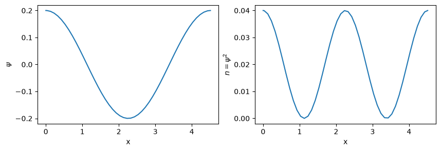
This subset of solutions can be found by direct integration starting from the initial condition that \(\psi_v(0)>0\) is the maximum of the wave with \(\psi_V'(0) = 0\). Since the wave must be convex at this point, we must have:
We thus have a continuous family of solutions with \(0 < \psi_V(0) < \sqrt{\mu/g}\).
Numerical Example#
Here we numerically solve this equation using the scipy IVP solver, then compare this with our exact solution as implemented in the gpe.exact_solutions.TravellingWave class.
from scipy.integrate import solve_ivp

class ODE:
    hbar = 1.0
    g = 1.0
    mu = 1.0
    m = 1.0

    @property
    def psi_max(self):
        if self.mu/self.g > 0:
            return np.sqrt(self.mu/self.g)
        else:
            return 1.0

    def f(self, x, y):
        psi, dpsi = y
        ddpsi = 2*self.m*(self.g*np.abs(psi)**2 - self.mu)*psi/self.hbar**2
        return (dpsi, ddpsi)

    def event(self, x, y):
        """Termination when dpsi=0 again"""
        if x <= 0:
            return -1
        psi, dpsi = y
        return dpsi

    event.terminal = True
    event.direction = -1

    def solve(self, fraction=0.9, max_step=0.1):
        x_max = 10.0
        psi0 = fraction*self.psi_max
        ivp = solve_ivp(self.f, (0, x_max), (psi0, 0),
                        max_step=max_step, events=[self.event])
        return ivp


ode = ODE()
ivp = ode.solve(0.2)
x, psi = ivp.t, ivp.y[0]
plt.figure(figsize=(10,3))
ax1 = plt.subplot(121)
ax1.plot(x, psi)
ax1.set(xlabel="x", ylabel=r'$\psi$')
ax2 = plt.subplot(122)
ax2.plot(x, psi**2)
ax2.set(xlabel="x", ylabel=r'$n=\psi^2$')
L = ivp.t_events[0]
Here we construct the same solution from our exact solution.
# Note: there is some error in the period for longer waves.
from gpe.imports import *
from gpe.exact_solutions import TravellingWaves

n1 = (psi**2).max()
n0 = 1e-8  # Should be zero, but for numerical reasons we just make small.
s = TravellingWaves(n1=n1, n0=n0, g=ode.g, Lx=ivp.t[-1]/2.0)
s.plot()
plt.plot(ivp.t-s.Lx/2, ivp.y[0]**2)
print("psi_0/sqrt(mu/g) = {}".format(np.sqrt(n1/(s.get_mu().real/s.g))))
[I 20:02:11 numexpr.utils] NumExpr defaulting to 2 threads.
[I 20:02:11 root] Patching zope.interface.document.asReStructuredText to format code
---------------------------------------------------------------------------
KeyboardInterrupt                         Traceback (most recent call last)
Cell In[3], line 7
      3 from gpe.exact_solutions import TravellingWaves
      4
      5 n1 = (psi**2).max()
      6 n0 = 1e-8  # Should be zero, but for numerical reasons we just make small.
----> 7 s = TravellingWaves(n1=n1, n0=n0, g=ode.g, Lx=ivp.t[-1]/2.0)
      8 s.plot()
      9 plt.plot(ivp.t-s.Lx/2, ivp.y[0]**2)
     10 print("psi_0/sqrt(mu/g) = {}".format(np.sqrt(n1/(s.get_mu().real/s.g))))

File ~/checkouts/readthedocs.org/user_builds/gpe/checkouts/latest/src/gpe/exact_solutions.py:191, in TravellingWaves.__init__(self, Nx, Lx, n0, n1, m, g, hbar, v_p, v_x, twist, **kw)
    189 if twist is None:
    190     x = np.linspace(-Lx / 2.0, Lx / 2.0, 10000)
--> 191     _psi, twist = self.psi_exact(x=x, Lx=Lx)
    192 self._twist = twist
    194 if v_x is None:

File ~/checkouts/readthedocs.org/user_builds/gpe/checkouts/latest/src/gpe/exact_solutions.py:230, in TravellingWaves.psi_exact(self, x, Lx)
    228 theta = [0]
    229 for _n in range(1, len(x)):
--> 230     theta.append(theta[-1] + scipy.integrate.quad(dtheta, x[_n - 1], x[_n])[0])
    231 theta = np.array(theta)
    232 theta -= theta[len(x) // 2]

File ~/checkouts/readthedocs.org/user_builds/gpe/conda/latest/lib/python3.14/site-packages/scipy/integrate/_quadpack_py.py:479, in quad(func, a, b, args, full_output, epsabs, epsrel, limit, points, weight, wvar, wopts, maxp1, limlst, complex_func)
    476     return retval
    478 if weight is None:
--> 479     retval = _quad(func, a, b, args, full_output, epsabs, epsrel, limit,
    480                    points)
    481 else:
    482     if points is not None:

File ~/checkouts/readthedocs.org/user_builds/gpe/conda/latest/lib/python3.14/site-packages/scipy/integrate/_quadpack_py.py:626, in _quad(func, a, b, args, full_output, epsabs, epsrel, limit, points)
    624 if points is None:
    625     if infbounds == 0:
--> 626         return _quadpack._qagse(func,a,b,args,full_output,epsabs,epsrel,limit)
    627     else:
    628         return _quadpack._qagie(func, bound, infbounds, args, full_output,
    629                                 epsabs, epsrel, limit)

File ~/checkouts/readthedocs.org/user_builds/gpe/checkouts/latest/src/gpe/exact_solutions.py:225, in TravellingWaves.psi_exact.<locals>.dtheta(x)
    222 _a = self.v_p / self.v_unit
    223 C = self._C * self.n_unit
--> 225 def dtheta(x):
    226     return _a + C / self.n_exact(x)
    228 theta = [0]

KeyboardInterrupt:
Velocity of a Travelling Wave#
In the previous discussion, \(v\) is the phase velocity of the traveling wave. This is the velocity with which the peaks of the wave travel. In contrast, the group velocity determines how fast a wave packet will move, which is a different concept. This velocity, however, is frame dependent, and in general, we would prefer to characterize this with respect to some specific frames.
For waves with infinite wavelength on a non-zero background density (such as dark solitons, and some bright solitons), a preferred frame is defined by the background at infinity which is taken to be at rest.
For infinite-wavelength bright solitons with no background density, no preferred frame exists. By boosting, one can realize these solutions with any velocity.
For small amplitude oscillations (phonons), a preferred reference frame is defined by a stationary background density.
The question is how to define the preferred frame for large-amplitude, finite-wavelength modes. One possibility is to define the frame with no net current:
With this definition, we have phase velocity:
Hoefer and El#
We now consider the solution of Hoefer and El. They set \(\hbar=m=g=1\) so that we have the following units (in \(d=3\) dimensions):
Or, using the Madelung transform:
They express their solution in terms of four constants \(r_1\leq r_2\leq r_3\leq r_4\) which we can related to some more physical parameters such as the amplitude \(a\), minimum and maximum densities \(\rho_{\min,\max}\), period \(L\), and phase velocity \(V\);
We disagree with their definition of \(C\) which is:
Instead, we find
In our code, we would like to specify \(\rho_\min\), \(\rho_\max\), the period \(L\) and the phase velocity \(V\). To do this, we must solve for the Jacobi parameter \(m\):
import gpe.utils;reload(gpe.utils)
import gpe.bec;reload(gpe.bec)
from gpe.utils import evolve
import gpe.exact_solutions;reload(gpe.exact_solutions)
from gpe.exact_solutions import TravellingWaves

# v_p is the velocity of the constructed wave.
# v_x is the velocity of the frame.
s = TravellingWaves(Nx=64*2, Lx=10.0, n0=1.0, n1=1.1, v_p=0.5, v_x=0.5)
t_max = 10.0

for y in evolve(s, steps=500, dt_t_scale=0.5, t_max=t_max):
    plt.clf()
    y.plot()
The current is:
In the moving frame:
Thus, if \(\rho_V(x_v)\) is specified, then \(u_V(x_V) = C/\rho_V(x_V)\) will ensure that the conservation equation is satisfied if:
The solution of Hoefer and El can be can be expressed as (Note: \(k=\sqrt{m}\) for \(\sn(z,k)\) in some CASs. We use \(\sn(z;m)\) and \(K(m)\) here):
Note that, averaging over a complete period \(L = 2lK(m)\) is:
import gpe.utils;reload(gpe.utils)
import gpe.bec;reload(gpe.bec)
from gpe.utils import evolve
import gpe.exact_solutions;reload(gpe.exact_solutions)
from gpe.exact_solutions import BrightSoliton

s = BrightSoliton(Nx=64, Lx=10.0,
                  v=0.0, # v=10.0
                  v_x=10.0)
t_max = s.basis.Lxyz[0]/abs(s.v_x)

for y in evolve(s, steps=500, t_max=t_max):
    plt.clf()
    y.plot()
Reformulation#
Here we present a reformulation of the coefficients into more physically meaningful parameters. We start with the
This form immediately satisfies the continuity equation as long as \(\rho(x_v) = \rho(x-vt)\):
Next we have:
%pylab inline --no-import-all
from gpe.exact_solutions import sn, K
m = 0.999999999
L = 2*K(m)
x = np.linspace(-L,L,100)
plt.plot(x, sn(x, m)**2)
import numpy as np
np.random.seed(1)
r = np.random.random(5)
r[4] = -r[1]-r[2]-r[3]
C = 1./8*(-r[1]-r[2]+r[3]+r[4])*(-r[1]+r[2]-r[3]+r[4])*(r[1]-r[2]-r[3]+r[4])
V = (r[1]+r[2]+r[3]+r[4])/2
m = (r[2]-r[1])*(r[4]-r[3])/(r[4]-r[2])/(r[3]-r[1])
k = np.sqrt(m)
a = (r[4]-r[3])*(r[2]-r[1])
l = 1./np.sqrt((r[4]-r[2])*(r[3]-r[1]))
rho_min = (r[1]-r[2]-r[3]+r[4])**2
rho_max = rho_min + a
V, np.sqrt(rho_min*rho_max*(1+rho_min*l**2))/l, C
Phonon Limit#
In the limit of small amplitude \(a\) we have the following reduction:
\omega(q) = \pm\sqrt{q^2(\rho_0 + q^2/4)}, \qquad V_p = \frac{\omega(q)}{q} = \pm\sqrt{\rho_0 + q^2/4}, \qquad V_g = \omega’(q) = \frac{q^2+2\rho_0}{\pm\sqrt{q^2 + 4\rho_0}} $$
Thus, one can specify the following four parameters (and an overall arbitrary initial phase):
\(\rho_\min\) and \(\rho_\max\): These determine the amplitude \(a = \rho_\max - \rho_\min \geq 0\) of the wave.
\(L\): The period of the wave can be chosen implicitly by setting \(l\) which will determine the period through \(m=al^2\) and \(L = 2l K(m)\).
\(V\): The speed of the wave may also be arbitrarily chosen. This may seem strange since the speed of the waves should follow from the dispersion relationship, however, this is simply a reflection of the fact that we can look at the system in an arbitrarily moving frame.
The rest frame is defined as the frame in which there is no net momentum flow. Thus, the average current should be zero:
\[\begin{split} 0 = \bar{\vect{j}} = \frac{1}{L}\int_0^L \vect{j}(x, t)\d{x} = \frac{1}{L}\int_0^L \rho(x, t)u(x, t)\d{x} = \frac{1}{L}\int_0^L \Bigl(V\rho(x, t) - C\Bigr)\d{x}\\ V_p = \frac{CL}{\int_0^L \rho(x, t)\d{x}} = \frac{C}{\bar{\rho}} \end{split}\]where \(\bar{\rho}\) is the average density across the cell. Note: this depiction will fail for bright solitons on the vacuum since \(\bar{\rho} = 0\) but in this case, the notion of the fixed background has no meaning.
Soliton Limit#
In the long wavelength limit \(m \rightarrow 1\):
Thus, the speed of the traveling waves is set by the minimum density in the long wavelength limit. This is consistent, for example, with the speed of a grey soliton which becomes stationary when it becomes dark (i.e. when the minimum density in the soliton becomes zero.)
from gpe.imports import *
import gpe.exact_solutions; reload(gpe.exact_solutions)
from gpe.exact_solutions import TravellingWaves

s = TravellingWaves(v_p=10.0, v_x=10.0, n0=0.1, Nx=32*4, Lx=5)
s.plot()
t_max = s.basis.Lxyz[0]/abs(s.v_p)

for y in evolve(s, steps=400, t_max=t_max):
    plt.clf()
    y.plot()
from gpe.imports import *
#from mmfutils.math.special import ellipkinv
from scipy.special import ellipj, ellipk
import scipy.integrate
import scipy as sp
import gpe.bec

def sn(u, m):
    return ellipj(u, m)[0]

def K(m):
    return ellipk(m)


def get_QV(m=0.1, a=0.1, rho_min=1.0, N=256):
    rho_max = rho_min + a
    #m = a*l**2
    l = np.sqrt(m/a)
    L = 2*l*K(m)
    dx = L/N
    x = np.arange(N)*dx
    rho = rho_min + a*sn(x/l, m)**2
    C = np.sqrt(rho_min*rho_max*(1+rho_min*l**2))/l
    V = np.trapz(C/rho, x)/L
    Q = 2*np.pi/L
    return Q, V

rho_min = 1.0
c = np.sqrt(rho_min)
ms = 1 - 10**np.linspace(-10, -0.001, 1000)

plt.figure(figsize=(20,5))
ax1 = plt.subplot(121)
ax2 = plt.subplot(122)
for a in [0.01, 0.2, 1.0]:
    Q, Vp = np.array([get_QV(m, a=a, rho_min=rho_min) for m in ms]).T
    l, = ax1.plot(Q**2, Vp/c, '-+', label=a)
    Q_ = (Q[1:]+Q[:-1])/2
    Vp_ = (Vp[1:]+Vp[:-1])/2
    Vg_ = Q_*np.diff(Vp)/np.diff(Q) +Vp_
    ax1.plot(Q_**2, Vg_/c, '--', c=l.get_c())

    ax2.plot(Q, Q*Vp, '-+', label=a)

q_max = 2.0
q = np.sqrt(np.linspace(0, q_max**2, 100))
Vp = np.sqrt(rho_min + q**2/4)
w = Vp*q
Vg = (q**2 +2*rho_min)/np.sqrt(q**2 +4*rho_min)
l, = ax1.plot(q**2, Vp/c, label='phonon')
ax1.plot(q**2, Vg/c, '--', c=l.get_c())
ax1.set_xlim(0, q_max**2)
ax1.set_ylim(0.99, 1.5)
plt.sca(ax1)
plt.axis([0,1.5,1,1.5])
ax1.set_xlabel("$q^2$")
ax1.legend()

plt.sca(ax2)
ax2.plot(q, w, label='phonon')
ax2.set_xlabel("$q$")
ax2.set_ylabel("$\omega(q)$")
ax2.set_xlim(0, 1.25)
ax2.set_ylim(0, 2)
#plt.axis([0,0.5,0,0.5])
ax2.legend()


get_QV(m=0.9999999999999999, a=1.0)
1.15*2.0
from gpe.soc import u
L = 2.5/3.0*u.micron
g = 0.00077
m = 87*u.u
hbar = u.hbar
u_length = g/hbar**2*m
Q = 2*np.pi/(L/u_length)
rho_max = 10530.0/u.micron**3*u_length**3
rho_min = 452.0/u.micron**3*u_length**3
a = rho_max - rho_min
get_QV(m=0.999999992, a=a)
from gpe.imports import *
import scipy.optimize
from scipy.special import ellipj, ellipk
import scipy.integrate
import scipy as sp
import gpe.bec

def sn(u, m):
    return ellipj(u, m)[0]

def cn(u, m):
    return ellipj(u, m)[0]

def K(m):
    return ellipk(m)

def get_m(a, L):
    def f(m):
        return 2*np.sqrt(m/a)*K(m) - L

    m0 = m1 = 0
    f0 = f1 = f(m0)
    while f1 < 0:
        m1 = (m1 + 1)/2.0
        f1 = f(m1)
    return sp.optimize.brentq(f, m0, m1)
class State(gpe.bec.State):
    def __init__(self, Nx=256, cells_x=10,
                 l=1.1757305, b=1.0, a=0.1, V=0.0):
        m = a*l**2
        L = 2*l*K(m) * cells_x
        mu = ((a+3*b)*l**2+1)/2/l**2
        C = np.sqrt((a+b)*b*(1+b*l**2)/l**2)
        dx = L/Nx
        gpe.bec.State.__init__(self, Nxyz=(Nx,), Lxyz=(L,),
                               m=1.0, g=1.0, hbar=1.0)

        x = self.basis.xyz[0]
        rho = b + a*sn(x/l, m)**2
        u = V - C/rho
        psi = np.sqrt(rho)*np.exp(1j*sp.integrate.cumtrapz(u, x, initial=0))
        self.data[...] = psi
        # Hpsi = np.fft.ifft(k**2*np.fft.fft(psi))/2 + (abs(psi)**2-mu)*psi
        #plt.plot(x, abs(Hpsi))

    def get_Vext(self):
        return 0.0

s = State(Nx=256)

e = EvolverABM(s, dt=0.5*s.t_scale)
with NoInterrupt() as interrupted:
    while not interrupted:
        e.evolve(100)
        e.y.plot()
        display(plt.gcf())
        plt.close('all')
        clear_output(wait=True)
import scipy.integrate
import scipy as sp

l = 1.1858
l = 1.1757305
b = 1.0
a = 0.1
V = 0.0
m = a*l**2
L = 2*l*K(m)
mu = ((a+3*b)*l**2+1)/2/l**2
C = np.sqrt((a+b)*b*(1+b*l**2)/l**2)
N = 256
dx = 10*L/N
x = np.arange(N)*dx - L/2
k = 2*np.pi * np.fft.fftfreq(N, dx)
rho = b + a*sn(x/l, m)**2
u = V - C/rho
#plt.plot(x, rho)
psi = np.sqrt(rho)*np.exp(1j*sp.integrate.cumtrapz(u, x, initial=0))
Hpsi = np.fft.ifft(k**2*np.fft.fft(psi))/2 + (abs(psi)**2-mu)*psi
plt.plot(x, abs(Hpsi))
plt.plot(x, rho*u**2 + rho**2/2)
plt.plot(x[1:-1], 2.36+rho[1:-1]*np.diff(np.diff(np.log(rho)))/dx**2/4)
from gpe.imports import *
from gpe.bec import State
s =
#
Phonons#
Phonons appear in the small amplitude limit \(a\rightarrow 0\) in which case:
The phase velocity is \(V = \omega(Q)/Q\)
and present the density as:
The soliton limit is \(m=1\) (i.e. \(r_2=r_3\)) where \(\sn(z, 1) = \tanh(z)\) where the solution has the form:
A traveling wave with velocity \(v\) has the following form:
By appropriately adjusting \(\mu\) we may set \(\omega = 0\), hence we may drop the factor \(e^{-\I\omega t}\) from the wavefunction:
The last equation above now represents a stationary solution in a moving frame with coordinate \(y = x-vt\):
where \(p_v = mv\). Finally, we may recast this in terms of the original GPE by transforming \(\psi(y)\) as follows:
If the original function \(\psi(y+L) = \psi(y)\) was periodic, then \(\tilde{\psi}(y+L) = e^{\I p_v L/\hbar}\tilde{\psi}(y)\). In other words, twisted boundary conditions should be applied with a twist \(\theta = p_vL/\hbar\).
GPE#
Here we consider the problem of finding traveling wave solutions in a BEC. From a numerical perspective, it is highly beneficial if the problem can be stated in terms of a well-defined minimization problem. To start, we consider the available analytic solution for the conventional GPE. These solutions are presented in [El:2016]:
The physical interpretations are:
\(a\): Amplitude
\(v\): Phase velocity
\(u\):
A special limit is when \(m=1\):
First we test these. To match units we set \(\hbar = m = g = 1\).
from gpe.imports import *
from scipy.special import ellipj, ellipk
import gpe.bec

def sn(u, m):
    return ellipj(u, m)[0]

def cn(u, m):
    return ellipj(u, m)[0]

def K(m):
    return ellipk(m)

class State(gpe.bec.State):
    def __init__(self, Nx=32, rs=[0.1, 0.2, 0.3, 0.4], xi0=0):
        r1, r2, r3, r4 = rs = sorted(rs)
        k = np.sqrt((r4-r2)*(r3-r1))
        m = (r2-r1)*(r4-r3)/(r4-r2)/(r3-r1)
        v = sum(rs)/2.0
        L = 2.*K(m)/k
        gpe.bec.State.__init__(self, Nxyz=(Nx,), Lxyz=(L,),
                               m=1.0, g=1.0, hbar=1.0)
        x = self.xyz[0]
        self.T = abs(L/v)
        t = 0
        xi = x - v*t - xi0
        a = (r4-r3)*(r2-r1)
        #a = m**2*k**2
        rho_0 = (r4-r3-r2+r1)**2/4.0
        rho_0 = (r4-r3+r2-r1)**2/4.0
        rho = rho_0  + a*sn(k*xi, m)**2
        self.a_ = self.a = a
        self.m_ = m
        self.k_ = self.k = k
        self.rho_0_ = self.rho_0 = rho_0

        k_ = self.m*v/self.hbar
        self[...] = np.exp(1j*k_*x) * np.sqrt(rho)

    def get_Vext(self):
        return 0.0

s = State(Nx=256, rs=[-2.0, -1.0, 1.0, 2.0])
n = s.get_density()
x = s.xyz[0]
x_ = x[1:-1]
psi_ = s[1:-1]
ddpsi_ = np.diff(np.diff(s[...]))/np.diff(x)[1:]**2
plt.plot(x_, ddpsi_/psi_/2 + abs(psi_)**2)
Check the soliton limit (2.122)
s = State(Nx=128, rs=[-4.000001, 1.0, 1.000001, 2.0])
x = s.xyz[0]
s.plot()
rho_min = abs(s[...]).min()**2
rho_max = abs(s[...]).max()**2
plt.axhspan(rho_min, rho_min + s.a, fc='y', alpha=0.5)
#plt.plot(x, rho_max-s.a/np.cosh(np.sqrt(s.a)*x)**2, '+:')
rho_0 = s.rho_0
s[...] = np.sqrt(rho_0)*np.tanh(np.sqrt(rho_0)*x)
s.plot()
s.cooling_phase = 1
e = EvolverABM(s, dt=0.9*s.t_scale)

with NoInterrupt(ignore=True) as interrupted:
    while e.t < e.y.T and not interrupted:
        e.evolve(100)
        plt.clf()
        e.y.plot()
        display(plt.gcf())
        clear_output(wait=True)
Solitons#
The GPE admits grey solitons with infinite period. These solitons arise from the previous solutions in the limit where \(m\rightarrow 1\) so that \(\sn\rightarrow\tanh\) and \(\cn\rightarrow\dn\rightarrow \sech\).
The soliton solution is:
This can be expressed as
or, in the same units \(m=\hbar = g = 1\) as El and Hoefer:
To compare with (2.117):
we have \(m=1\), \(\sn = \tanh\) and
Everything here is reasonable except the definition of the phase velocity \(V\) which differs from the soliton velocity \(v\).
The background density is
To compare with (2.122):
, the stationary solution must have \(\bar{\rho} = a_s\) or:
If \(r_1 = -r_4-2r_2\), then
Issues#
I was having some issues finding solutions so I considered stationary solutions:
Symbolically solving for solutions to the GPE (in Maple) gives the following solutions:
(assuming \(a,k\neq 0\) and real \(k\)) gives:
restart;
X_:=JacobiSN(k*x,sqrt(m2));
psi:=sqrt(rho[0] + a*X_^2);
Rho:=psi^2:
res:=collect(numer(simplify(-diff(psi, x, x)/2/psi + Rho - mu)), X_):
mu:=expand(solve(coeff(res, X_, 0), mu));
m2:=solve(coeff(res, X_^6), m2);
solve([coeffs(res, X_)], [a,k^2]);
The dark soliton solution has \(m=1\), \(a=k^2\)
s.m
s = State(rs=[-4.1, 1.0, 1.1, 2.])
x = s.xyz[0]
m = s.m_
a = s.a_
k = s.k_
rho_0 = s.rho_0_
print(m, a, m**2*k**2, rho_0, k)
k = np.sqrt(rho_0)
plt.plot(x, 1+sn(k*x,m)**2)
#s[...] = np.sqrt(rho_0*(1-sn(x,m)))
To do this, we first consider boosting to a moving frame with velocity \(v\) so that in this frame, the traveling wave solution is stationary and periodic. We second Here we are looking for solutions that satisfy:
Minimization#
Here we consider the hypothesis that traveling waves can be found as minimum energy solutions in a box of period \(L\) with twisted boundary conditions holding both the total particle number fixed and the value of the wavefunction at one point.
We start with the soliton solution:
At the core, the density is:
from gpe.imports import *
import gpe.Examples.traveling_waves;reload(gpe.Examples.traveling_waves)
from gpe.Examples.traveling_waves import (
    StateTravellingWave, MinimizeStateTravellingWave)
from gpe.exact_solutions import TravellingWaves

n1 = 1.0
n0 = 0.5
tw0 = TravellingWaves(n1=n1, n0=0.5)
n_avg = tw0.get_density().mean()
s = StateTravellingWave(Nx=tw0.basis.Nx, Lx=tw0.basis.Lx,
                        psi_0=tw0[0], ind=0,
                        n_avg=n_avg, v_p=tw0.v_x, twist=tw0.twist)
s.set_psi(tw0.get_psi())
#s[...] = ts0[...]
s.cooling_phase = 1
e = EvolverABM(s, dt=0.1*s.t_scale, normalize=False)
with NoInterrupt() as interrupted:
    while not interrupted:
        e.evolve(200)
        plt.clf()
        e.y.plot()
        display(plt.gcf())
        clear_output(wait=True)
plt.plot(tw0.xyz[0], s[...] - tw0[...])
plt.plot(tw0.get_Vext()- s.get_Vext())
dy0 = tw0.empty()
tw0.compute_dy_dt(dy=dy0, subtract_mu=False)
dy = s.empty()
s.compute_dy_dt(dy=dy, subtract_mu=False)
dy0[...] - dy[...]
s.plot()
dy = s.empty()
s.compute_dy_dt(dy=dy)
s.cooling_phase = 1j

e = EvolverABM(s, dt=0.5*s.t_scale, normalize=True)
with NoInterrupt() as interrupted:
    while not interrupted:
        e.evolve(100)
        plt.clf()
        e.y.plot()
        display(plt.gcf())
        clear_output(wait=True)
from scipy.optimize import brentq
n1 = 1.0
n_avg = 0.9
def f(n0):
    print(n0)
    tw = TravellingWaves(n1=n1, n0=n0)
    return tw.get_density().mean() - n_avg
brentq(f, 0, n1*0.999)
from gpe.imports import *
import gpe.Examples.traveling_waves;reload(gpe.Examples.traveling_waves)
from gpe.Examples.traveling_waves import StateTravellingWave, MinimizeStateTravellingWave
vs = np.linspace(-1,1,10)
Es = []
for v in vs:
    s0 = StateTravellingWave(Nx=128, L=10.0, v_p=v, twist=0.1)
    m = MinimizeStateTravellingWave(s0)
    s = m.minimize()
    Es.append(s.get_energy())
    plt.clf()
    s.plot()
    display(plt.gcf())
    clear_output(wait=True)
plt.plot(vs, Es)
Here is a stationary dark soliton.
%%time
dark_soliton = Soliton()

s0 = StateTravellingWave(psi_0=0, twist=np.pi, v_p=0)
s0[...] = dark_soliton.get_psi(s0.xyz[0])

m = MinimizeStateTravellingWave(s0)
s = m.minimize(E_tol=1e-12, psi_tol=1e-12)
s.plot()
plt.plot(x, abs(dark_soliton.get_psi(x))**2, '--', label='exact')
plt.legend(loc='best')
grey_soliton = Soliton(v=0.999)
plt.plot(np.angle(grey_soliton.get_psi(s0.xyz[0])))
v_c = 0.1
np.arctan2(v_c, np.sqrt(1-v_c**2))
v_c = grey_soliton.v/grey_soliton.c
theta = np.arctan2(v_c, np.sqrt(1-v_c**2))
s0 = StateTravellingWave(psi_0=0, twist=np.pi+2*theta, v_p=grey_soliton.v)
s0[...] = grey_soliton.get_psi(s0.xyz[0])
s0.psi_0 = abs(s0[...]).min()

m = MinimizeStateTravellingWave(s0)
s = m.minimize(E_tol=1e-12, psi_tol=1e-12)
s.plot()
plt.plot(x, abs(grey_soliton.get_psi(x))**2, '--', label='exact')
plt.legend(loc='best')
Here is a moving grey soliton.
plt.plot(np.angle(s._twist_phase_x)/np.pi)
%%time
rho_min = 0.01
v_p = np.sqrt(s.g*rho_min/s.m)
s0 = StateTravellingWave(psi_0=np.sqrt(rho_min), twist=np.pi, v_p=v_p)
s0[...] = s[...]
m = MinimizeStateTravellingWave(s0)
s = m.minimize(E_tol=1e-12, psi_tol=1e-12)
s.plot()
Exact Solution#
from gpe.imports import *
#from mmfutils.math.special import ellipkinv
from scipy.special import ellipj, ellipk
import scipy.integrate
import scipy as sp
import gpe.bec

def sn(u, m):
    return ellipj(u, m)[0]

def K(m):
    return ellipk(m)


def get_QV(m=0.1, a=0.1, rho_min=1.0, N=256):
    rho_max = rho_min + a
    #m = a*l**2
    l = np.sqrt(m/a)
    L = 2*l*K(m)
    dx = L/N
    x = np.arange(N)*dx
    rho = rho_min + a*sn(x/l, m)**2
    C = np.sqrt(rho_min*rho_max*(1+rho_min*l**2))/l
    Vp = np.trapz(C/rho, x)/L
    Q = 2*np.pi/L
    return Q, Vp

rho_min = 1.0
a = 0.1
m = 0.63315
l = np.sqrt(m/a)
L = 2*l*K(m)
Q, Vp = get_QV(m=m, a=a, rho_min=rho_min)
x0 = m.pack(s0[...])
s0[...] = m.unpack(x0)
s0.plot()
s0 = State(Nx=64, L=L, mu=10.0, psi_0=np.sqrt(rho_min),
          v=Vp, m=1.0, hbar=1.0, g=1.0)
s0.plot()
plt.figure()
m = MinimizeState(s0, fix_N=True)
m.check()
s = m.minimize(psi_tol=1e-12, E_tol=1e-12)
s.plot()
s = State(Nx=128*8, L=120.0, mu=1.0, psi_0=0.5, v=v)
psi_s = s.exact_psi()
v = (np.angle(psi_s[-1]) - np.angle(psi_s[0])+np.pi)*s.hbar/s.m/(s.Lxyz[0] - s.Lxyz[0]/s.Nxyz[0])
s = State(Nx=128*8, L=120.0, mu=1.0, psi_0=0.5, v=v)
s[...] = s.exact_psi()
print(v)
plt.plot(s[...]/s.twist_phase)
v
s = s1
s.cooling_phase = 1.0
e = EvolverABM(s, dt=0.5*s.t_scale)

with NoInterrupt(ignore=True) as interrupted:
    while not interrupted:
        e.evolve(100)
        plt.clf()
        e.y.plot()
        display(plt.gcf())
        clear_output(wait=True)
s = State(Nx=128*4, L=20.0, mu=1.0, psi_0=0.1, v=0.1)
s[...] = 1.0
m = MinimizeState(s, fix_N=False)
s1 = m.minimize(use_scipy=True)
plt.plot(s1.xyz[0], s1.get_density() - abs(s1.exact_psi())**2)
#s1.plot()
abs(s1.get_density() - abs(s1.exact_psi())**2).max()
plt.plot(s1.xyz[0], np.angle(s1[...]))
plt.plot(s1.xyz[0], np.angle(s1.exact_psi()))
vs = np.linspace(0, 0.4, 10)
errs = []
for v in vs:
    s = State(Nx=128*4, L=20.0, mu=1.0, psi_0=0.2, v=v)
    m = MinimizeState(s, fix_N=False)
    s1 = m.minimize(use_scipy=True)
    errs.append(abs(s1.get_density() - abs(s1.exact_psi())**2).max())
New#
from gpe.Examples import traveling_waves

class StateCustomDisp(traveling_waves.StateTwist_x):
    def __init__(self, Nx=128, L=10.0, mu=1.0, psi_0=1.0, ind=None,
                 v_p=0.0, twist=0.0, m=1.0, hbar=1.0, g=1.0):
        """
        Arguments
        ---------

        """
        self.v_p = v_p
        if ind is None:
            ind = Nx//2
        self.ind = ind
        self.psi_0 = psi_0
        self.p_v = p_v = m*v_p
        twist_x = twist  # + p_v * L / hbar
        traveling_waves.StateTwist_x.__init__(self, Nxyz=(Nx,), Lxyz=(L,),
                              m=m, hbar=hbar, g=g,
                              mu=mu, twist_x=twist_x)
        self[self.ind] = psi_0

    def init(self):
        traveling_waves.StateTwist_x.init(self)
        self._kx2 = (self.get_dispersion() * 2. * self.m / self.hbar**2)**2

    def get_Vext(self):
        return 0

    def get_dispersion(self):
        k = self._kx
        disp = (k * self.hbar)**2 / 2. / self.m - self.v_p * k
        return disp
s.get_Vext()
s0 = StateCustomDisp(Nx=2**6, L=5, mu=1.0, psi_0=np.sqrt(0), v_p=0.1, twist=0)
m = MinimizeStateTravellingWave(s0)
s_init = m.minimize(E_tol=1e-12, psi_tol=1e-12)
def get_err(v_p, s_guess=[s_init]):
    s0 = StateCustomDisp(Nx=2**6, L=5, mu=1.0, psi_0=np.sqrt(0.1), v_p=v_p, twist=0)
    if s_guess[0] is not None:
        s0[...] = s_guess[0][...]
    m = MinimizeStateTravellingWave(s0)
    s = m.minimize(E_tol=1e-12, psi_tol=1e-12)
    s[s.ind] = s.psi_0
    s_guess[0] = s
    err = abs(s.compute_dy_dt(dy=s.copy())[...]).max()
    plt.clf()
    s.plot()
    plt.ylabel(v_p)
    plt.xlabel(err)
    display(plt.gcf())
    clear_output(wait=True)
    return err

v_ps = np.linspace(0,1,100)
errs = map(get_err, v_ps)
plt.plot(v_ps[1:], errs[1:])
v_p = 0.19
s0 = StateCustomDisp(Nx=2**6, L=10.0, mu=1.0, psi_0=np.sqrt(0.1), v_p=v_p, twist=0)
m = MinimizeStateTravellingWave(s0)
s = m.minimize(E_tol=1e-12, psi_tol=1e-12)
s.plot()
sp.integrate.cumtrapz?
n = s.get_density()
L = s.basis.Lx
x = s.basis.xyz[0]
rho_min = n.min()
rho_max = n.max()

def get_rho_v_p(L=5.0, rho_min=0.1, rho_max=1.2, x=None):
    if x is None:
        x = np.linspace(-L/2., L/2.0, 1000)
    a = rho_max - rho_min
    m = get_m(a=a, L=L)
    l = np.sqrt(m/a)
    rho = rho_min + a*sn(x/l, m)**2
    C = np.sqrt(rho_min*rho_max*(1.+rho_min*l**2))/l
    plt.plot(x, rho)
    v_p = np.trapz(C/rho, x)/L
    u = v_p - C/rho
    theta = sp.integrate.cumtrapz(u, x, initial=0)
    return lambda x:rho_min + a*sn(x/l, m)**2, v_p, theta
plt.plot(x, theta)
plt.plot(x, s0[...].real)
plt.plot(x, s0[...].imag)
L = 3.0
rho_max = 1.2
rho_min = 0.5

rho, v_p, theta = get_rho_v_p(L=L, rho_min=rho_min, rho_max=rho_max)

s0 = StateCustomDisp(Nx=2**7, L=L, mu=rho_max, psi_0=np.sqrt(rho_min), v_p=v_p, twist=0)
x = s0.basis.xyz[0]
rho, v_p, theta = get_rho_v_p(L=L, rho_min=rho_min, rho_max=rho_max, x=x)
s0[...] = np.sqrt(rho(s0.basis.xyz[0]))*np.exp(1j*theta)
N_tot = s0.get_N()
Nx = s.basis.Nx
#s0[...] = np.sqrt((N_tot*Nx/L  - rho_min)/(Nx-1))*np.exp(1j*s.m*x*v_p/s.hbar)
#s0[s0.ind] = s0.psi_0
#print(N_tot, s0.get_N())


m = MinimizeStateTravellingWave(s0)
s = m.minimize(E_tol=1e-12, psi_tol=1e-12)
m.check()
s.plot()
#print s[s.ind]/s.psi_0 - 1
dy = s0.compute_dy_dt(s0.copy())
plt.plot(x, abs(dy[...]))
abs(dy[...]).max()
s[s.ind] = s.psi_0
    s_guess[0] = s
    err = abs(s.compute_dy_dt(dy=s.copy())[...]).max()
    plt.clf()
    s.plot()
    plt.ylabel(v_p)
    plt.xlabel(err)
    display(plt.gcf())
    clear_output(wait=True)
    return err

v_ps = np.linspac
s0 = StateCustomDisp(Nx=2**6, L=10.0, mu=1.0, psi_0=np.sqrt(1.), v_p=0.1, twist=0.0)
m = MinimizeStateTravellingWave(s0)
s = m.minimize(E_tol=1e-12, psi_tol=1e-6)
s.plot()
plt.figure()
dy = s.copy()
dy = s.compute_dy_dt(dy=dy)
dy.plot()
dy = s.copy()
dy = s.compute_dy_dt(dy=dy)
plt.semilogy(abs(dy[...]))