import mmf_setup

mmf_setup.nbinit()
This cell adds /home/docs/checkouts/readthedocs.org/user_builds/gpe/checkouts/latest/src to your path, and contains some definitions for equations and some CSS for styling the notebook. If things look a bit strange, please try the following:
- Choose "Trust Notebook" from the "File" menu.
- Re-execute this cell.
- Reload the notebook.
Table of Contents
Fourier Transform#
The Fourier transform (FT) converts a function of position \(x\) or time \(t\) into a function of wavevector \(k\) or frequency \(\omega\):
Note that in quantum mechanics, the wavevector is related to the momentum \(p = \hbar k\) and the frequency is related to the energy \(E = \hbar \omega\) through the Planck constant \(\hbar\). In the following, we may refer to “momentum” in terms like “momentum space” when we should properly state “wavevector”. This is due to the common convention of considering \(\hbar\) as simply defining units. Instead, theoretical physicists often use units where \(\hbar = 1\).
The inverse transform is also well-defined:
Here we have used the normalization condition common in physics whereby a factor of \(1/2\pi\) is included with the momentum/frequency interval. This leads to a slight asymmetry in the inner product (see below) but has some nice behavior when taking the continuum limit of a finite basis.
This relationship is based on Parseval’s Theorem which leads to the following identities:
There are subtleties regarding the nature of the functions \(f(x)\) and \(f_k\) in order to render intervals convergent. For most (but not all) physical applications, these can be neglected. If in doubt, express the problem in a finite basis by inserting a cutoff or lattice, then take the continuum limit.
Linear Algebra#
This transformation can be thought of in terms of linear algebra as a change of basis. Here functions are vectors, and we have an inner product defined in terms of the integral:
The space of functions admits two bases: the position basis \(\ket{x}\) and the momentum basis \(\ket{x}\) such that:
In terms of the position basis, the momentum basis consists of plane waves. Expressed in this way, the Fourier transform is simply a change of basis and can be implemented in terms of the following resolutions of unity:
To effect one of the transformations, simply insert the appropriate form of the identity. I.e., for the inverse transform:
Discrete Fourier Transform#
The Fourier transformation discussed above is formulated in terms of the full set of continuous positions \(x \in (-\infty, \infty)\). There are two useful restrictions. The first is to consider periodic functions \(f(x+L) = f(x)\) which can be restricted to the fixed interval \(x \in [0, L)\). In this case, the momenta no longer take continuous values, but are instead restricted to the values:
where \(m\) is an integer. These functions are now expressed in terms of a Fourier series:
Less frequently used, the second restriction is to consider a function tabulated only on a discrete set of lattice points in position space with lattice spacing \(\d{x}\):
Now the momenta are continuous but limited to a finite interval \(k \in [-\pi/\d{x}, \pi/\d{x})\):
In this case, the functions of momenta are periodic \(f_{k + 2\pi/\d{x}} = f_k\).
Combining these, we obtain a fully discrete and finite basis with \(N\) equally spaced points with spacing \(\d{x} = L/N\) on an interval of length \(L\). I use conventionally use the following lattice and momentum points:
One can easily represent the discrete Fourier transform (DFT) in analogy with the continuous Fourier transform through the following table of correspondences. In addition, we include the usual normalization used for numerical work as implemented by the Fast Fourier Transform (FFT) to be discussed below. Since numbers are dimensionless, these are found by setting \(L=N\) – i.e. by taking a unit lattice spacing \(\d{x} = L/N = 1\).
Continuous (FT) |
Discrete (DFT) |
Finite (FFT) |
|---|---|---|
\(x\) |
\(x_n = \frac{L}{N} n \) |
\(n\in \{0, 1, \dots, N-1\}\) |
\(k\) |
\(k_m = \frac{2\pi}{L} m \) |
\(m\in \left\{0, 1, \dots, \frac{N}{2}-1,-\frac{N}{2}, -\frac{N}{2} + 1, \dots, -1\right\}\) |
\(\d{x}\) |
\(\frac{L}{N}\) |
\(1\) |
\(\frac{\d{k}}{2\pi}\) |
\(\frac{1}{L}\) |
\(\frac{1}{N}\) |
\(f(x)\) |
\(f_n = f(x_n)\) |
\(f_n\) |
\(f_k\) |
\(f_m = f_{k_m}\) |
\(f_m\) |
\(\int_{-\infty}^{\infty} \d{x}\) |
\(\frac{L}{N}\sum_{n=0}^{N-1}\) |
\(\sum_{n=0}^{N-1}\) |
\(\int_{-\infty}^{\infty} \frac{\d{k}}{2\pi}\) |
\(\frac{1}{L}\sum_{m=N/2}^{N/2-1}\) |
\(\frac{1}{N}\sum_{m=N/2}^{N/2-1}\) |
$\braket{x |
k} = e^{\I k x}$ |
$\braket{x_n |
\(f_k = \int_{-\infty}^{\infty} \d{x} e^{-\I k x} f(x)\) |
\(f_m = \frac{L}{N}\sum_{n=0}^{N-1} e^{-\I k_m x_n} f_n\) |
\(f_m = \sum_{n=0}^{N-1} e^{-2\pi \I m n/N} f_n\) |
\(f(x) = \int_{-\infty}^{\infty} \frac{\d{k}}{2\pi} e^{\I k x} f_k\) |
\(f_n = \frac{1}{L}\sum_{n=N/2}^{N/2-1} e^{\I k_m x_n} f_m\) |
\(f_n = \frac{1}{N}\sum_{n=N/2}^{N/2-1} e^{2\pi \I m n/N} f_m\) |
For the FFT, note that the order of the wavevector indices \(m\) which is rather specific, which corresponds with an efficient ordering for the numerical implementations. In some implementations, such as the underlying FFTW, the normalizing factor \(1/N\) in the IFFT is not computed for performance reasons and must be supplied by the user if needed. Other than this point, the conventions given here agree with both NumPy and FFTW implementations.
import numpy.fft, numpy as np

N = 64
L = 1.0
n = np.arange(N)
m = np.asarray(list(range(0, N // 2)) + list(range(-N // 2, 0)))
FFT = np.exp(-2 * np.pi * 1j * m[:, None] * n[None, :] / N)
IFFT = 1.0 / N * np.exp(2 * np.pi * 1j * m[None, :] * n[:, None] / N)

f_n = np.random.random(N) + 1j * np.random.random(N) - 0.5 - 0.5j
f_m = FFT.dot(f_n)
assert np.allclose(np.fft.fft(f_n), FFT.dot(f_n))
assert np.allclose(np.fft.ifft(f_m), IFFT.dot(f_m))
Let us consider a sequence \(u\) of \(N\) elements:
The discrete Fourier transformation of \(u\) is a sequence \(U\), whose elements \(U_k\) are given by
Compactly, \(U = D(u)\); where the symbol \(D()\) represents the discrete Fourier transformation of its argument.
We know that \(1\) has \(N\) \(N^{th}\) roots denoted by \(\omega_k\), \(k = 0, 1, 2, 3, \cdots \cdots, N-1\); where \(\omega_k = e^{\frac{2\pi i k}{N}}\). Therefore,
Properties of DFT#
Linearity: \(D(\alpha v + \beta w) = \alpha \, D(v) + \beta \, D(w); \quad v, w \in u; \, \alpha, \beta \in \mathbb{C}\).
Periodicity: \(U_{k + N} = U_k\)
Proof:
Inverse Discrete Fourier Transformation (IDFT)#
If we are given \(U = \left[U_t \right]_{t = 0}^{N-1}\), then the inverse discrete Fourier transformation of \(U\) is defined as
A Basis for Wavefunctions#
This machinery provides an efficient way of representing wavefunctions on a discrete lattice of \(N\) points over a periodic interval of length \(L\). As long as the functions to be represented are analytic and periodic (i.e. no kinks), then one typically enjoys exponential convergence properties.
Derivatives#
The utility of this basis comes in computing derivatives:
This is simply an expression of the fact that the derivative operator is diagonal in the momentum basis:
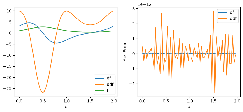
Here we demonstrate this by computing the first two derivatives of the following analytic and periodic function:
%pylab inline --no-import-all
import numpy.fft, numpy as np

N = 64
L = 2.0
dx = L / N
x = np.arange(N) * dx
k = 2 * np.pi * np.fft.fftfreq(N, dx)


def diff(f, d=1):
    """Return the d'th derivative of f"""
    return np.fft.ifft((1j * k) ** d * np.fft.fft(f))


arg = 2 * np.pi * x / L
f = np.exp(np.sin(arg))
df = 2 * np.pi / L * f * np.cos(arg)
ddf = (2 * np.pi / L) ** 2 * f * (np.cos(arg) ** 2 - np.sin(arg))

plt.figure(figsize=(10, 4))
plt.subplot(121)
plt.plot(x, df, label="df")
plt.plot(x, ddf, label="ddf")
plt.plot(x, f, label="f")
plt.xlabel("x")
plt.legend(loc="best")

plt.subplot(122)
plt.plot(x, df - diff(f, 1), "-", label="df")
plt.plot(x, ddf - diff(f, 2), "-", label="ddf")
plt.legend(loc="best")
plt.xlabel("x")
plt.ylabel("Abs Error")
%pylab is deprecated, use %matplotlib inline and import the required libraries.
Populating the interactive namespace from numpy and matplotlib
/home/docs/checkouts/readthedocs.org/user_builds/gpe/conda/latest/lib/python3.14/site-packages/matplotlib/cbook.py:1810: ComplexWarning: Casting complex values to real discards the imaginary part
  return math.isfinite(val)
/home/docs/checkouts/readthedocs.org/user_builds/gpe/conda/latest/lib/python3.14/site-packages/matplotlib/cbook.py:1407: ComplexWarning: Casting complex values to real discards the imaginary part
  return np.asanyarray(x, float)
Text(0, 0.5, 'Abs Error')
Convergence#
The convergence properties of the basis depend on two factors:
Infrared (IR) convergence: That the function is periodic (i.e. that it fits in the box).
Ultraviolet (UV) convergence: That the function is smooth enough to be properly represented by the finite lattice spacing.
Infrared (IR)#
The first type of convergence is called infrared (IR) convergence as the finite size of the box does not permit the study of arbitrarily long-wavelength modes (recall that IR light has a longer wavelength than visible light). The limitation here is that the box size \(L\) might be too small to represent large features of a problem.
Ultraviolet (UV)#
The second type of convergence is called ultraviolet (UV) convergence since the lattice is not fine enough to properly represent high-frequency components with \(\abs{k} > k_c = \pi N/L\). Since most objects obey a dispersion like \(E(p) = p^2/2m\), these features have low energy, so this is referred to as a high-energy cutoff \(E_c = \hbar^2 k_c^2/2m\).
Example#
We demonstrate this by considering the derivative of a Gaussian in a centered box:
To achieve machine precision (\(\epsilon = 2^{-52} \approx 2\times 10^{-16}\) for double precision), the function must:
Fit in the box. The appropriate condition is that \(f(L/2) < \epsilon \max(f)\), so we have the condition:
\[ L > \sigma\sqrt{-8\ln\epsilon} \approx 17\sigma. \]Not wiggle too fast. Here we express a similar condition on the Fourier transform \(f_{k_c} < \epsilon \max(f_k)\):
\[ k_c = \pi \frac{N}{L} > \sigma^{-1}\sqrt{-2\ln\epsilon}, \qquad N > \frac{L}{\sigma}\frac{\sqrt{-2\ln\epsilon}}{\pi} \approx 2.7\frac{L}{\sigma}. \]
Thus, for a Guassian, we require about \(N > 2.7\times 17 \approx 46 \) points to achieve accuracy to machine precision.
%pylab inline --no-import-all
from IPython.display import Latex


def f(x, sigma=1.0):
    return np.exp(-(x**2) / 2 / sigma**2)


def df(x, sigma=1.0):
    return -x / sigma**2 * f(x, sigma=sigma)


def get_error(N, L, sigma=1.0):
    dx = L / N
    x = np.arange(N) * dx - L / 2
    k = 2 * np.pi * np.fft.fftfreq(N, dx)
    _f = f(x, sigma)
    _df = df(x, sigma)
    dft = np.fft.ifft((1j * k) * np.fft.fft(_f))
    err = _df - dft
    return abs(err / abs(_df).max()).max()


eps = np.finfo(float).eps
display(Latex(r"$\epsilon =$ {}".format(eps)))
sigma = 1.0
L = np.sqrt(-8 * np.log(eps)) * sigma
N = int(np.ceil(np.sqrt(-2 * np.log(eps)) / np.pi * L / sigma))
print("Optimal N, L = ({}, {})".format(N, L))
%pylab is deprecated, use %matplotlib inline and import the required libraries.
Populating the interactive namespace from numpy and matplotlib
Optimal N, L = (46, 16.980848833699017)
Here we demonstrate that these are indeed optimal by computing the error in the derivative.
plt.figure(figsize=(10, 5))
plt.subplot(121)
Ns = np.arange(4, 60)
errs = [get_error(_N, L, sigma) for _N in Ns]
plt.semilogy(Ns, errs)
plt.xlabel("N")
plt.ylabel("Relative error in derivative")

plt.subplot(122)
Ls = np.linspace(L / 2, 1.5 * L, 100)
errs = [get_error(N, _L, sigma) for _L in Ls]
plt.semilogy(Ls, errs)
plt.xlabel(r"$L/\sigma$")
Text(0.5, 0, '$L/\\sigma$')
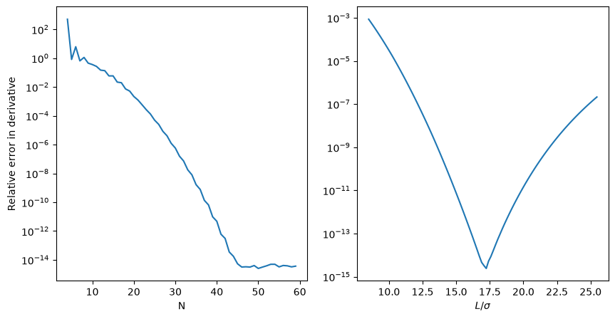
Notice that increasing the box size also increases the error. This is because we are holding the number of points \(N\) fixed, so increasing the box size also decreases the maximum momentum \(k_c\), thus the error for small \(L\) is IR while the error for larger \(L\) is UV. In the plot on the right, computational cost does not increases while it does in the plot to the left.
Twisted Boundary Conditions#
The periodic nature of the boundary conditions can be relaxed somewhat by allowing for a phase twist:
This twisted boundary conditions can be implemented with similar code by forming the periodic functions:
The FFT can then be applied to the functions \(\tilde{f}\). Note that to compute derivatives etc., one should multiply by the shifted momentum
Here we demonstrate the two steps required to compute the derivative of a function with twisted boundary conditions.
Example#
We demonstrate this by considering the derivative of a Gaussian in a centered box with a twist \(\theta = k_B L\):
%pylab inline --no-import-all
from IPython.display import Latex
from numpy.fft import fft, ifft, fftfreq


def f(x, sigma=1.0, k_B=1.0):
    return np.exp(1j * k_B * x - x**2 / 2 / sigma**2)


def df(x, sigma=1.0, k_B=1.0):
    return (1j * k_B - x / sigma**2) * f(x, sigma, k_B)


def get_error(N, L, sigma=1.0, theta=1.0):
    k_B = theta / L  # This is the twist or Bloch momentum
    dx = L / N
    x = np.arange(N) * dx - L / 2
    k = 2 * np.pi * fftfreq(N, dx)
    k += k_B  # Shift momenta to accomodate twisted boundary conditions.
    _f = f(x, sigma, k_B)
    _df = df(x, sigma, k_B)
    ft = np.exp(-1j * k_B * x) * _f  # Unapply twist to make periodic function
    dft = ifft((1j * k) * fft(ft))
    dft = np.exp(1j * k_B * x) * dft  # Reapply twist
    err = _df - dft
    return abs(err / abs(_df).max()).max()


eps = np.finfo(float).eps
display(Latex(r"$\epsilon =$ {}".format(eps)))
sigma = 1.0
theta = 0.1
L = np.sqrt(-8 * np.log(eps)) * sigma
N = int(np.ceil(np.sqrt(-2 * np.log(eps)) / np.pi * L / sigma))
print("Optimal N, L = ({}, {})".format(N, L))
%pylab is deprecated, use %matplotlib inline and import the required libraries.
Populating the interactive namespace from numpy and matplotlib
Optimal N, L = (46, 16.980848833699017)
N = 46
sigma = 1.0
theta = 1.0
L = 17.0
dx = L / N
x = np.arange(N) * dx - L / 2
k_B = theta / L
k = 2 * np.pi * np.fft.fftfreq(N, dx) + k_B
_f = f(x, sigma, k_B)
_df = df(x, sigma, k_B)
ft = np.exp(-1j * k_B * x) * _f
dft = np.exp(1j * k_B * x) * ifft(1j * k * fft(ft))
plt.figure(figsize=(10, 5))
plt.subplot(121)
Ns = np.arange(4, 60)
errs = [get_error(_N, L, sigma) for _N in Ns]
plt.semilogy(Ns, errs)
plt.xlabel("N")
plt.ylabel("Relative error in derivative")

plt.subplot(122)
Ls = np.linspace(L / 2, 1.5 * L, 100)
errs = [get_error(N, _L, sigma) for _L in Ls]
plt.semilogy(Ls, errs)
plt.xlabel(r"$L/\sigma$")
Text(0.5, 0, '$L/\\sigma$')
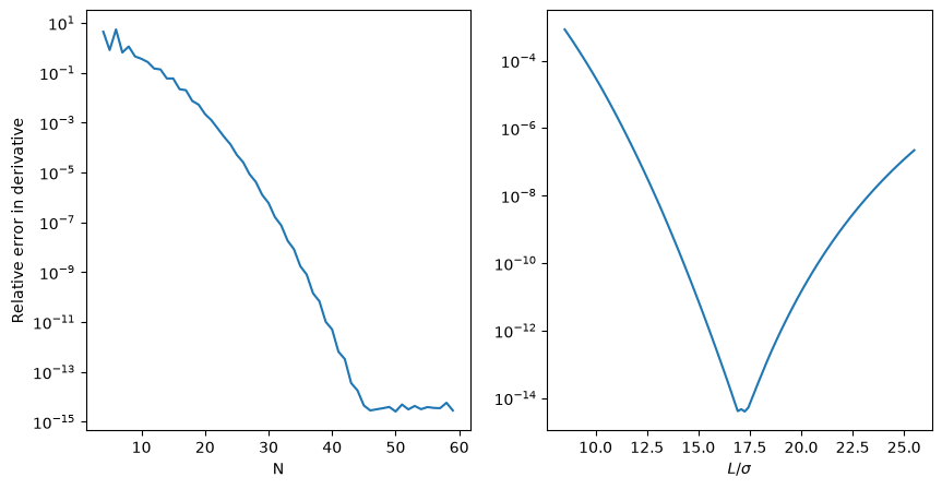
Notice that twisted boundary conditions allow you to explore momenta between the original discrete points \(k_m\). This is directly related to Bloch waves which is why we use \(k_B\), the “Bloch” momentum above. By averaging over all twists one can recover the physics of an infinite system with periodic structure which is different that physics in a strictly periodic universe where the momenta are indeed discrete.
Fast Fourier Transform (FFT)#
Outline#
import numpy as np
import matplotlib.pyplot as plt
When working on a lattice, one can use the homogeneous equations, by replacing the integral with a sum over lattice momenta. We give the explicit relationships here for a box of length \(L\) with \(N\) points and index \(n \in [0, 1, \cdots N-1]\). Note that the ordering of the indices \(m\) for \(k_m\) is different than listed because of how the FFT is implemented numerically. (See the following code for the explicit ordering.) The order listed can be obtained from this using np.fft.fftshift().
Here we have included the Bloch momentum \(k_B = \frac{\theta_B}{2\pi L}\) used when one implements a twist \(\pi/2 \leq \theta_B < \pi/2\) which acts to fill in the missing momenta.
import numpy as np
N, L = 8, 2.0
dx = L / N
x = np.arange(N) * dx - L / 2.0
k = 2 * np.pi * np.fft.fftfreq(N, dx)
m = (np.arange(N) + N // 2) % N - N // 2
k_ = 2 * np.pi * m / L
assert np.allclose(k, k_)
assert np.allclose(np.fft.fftshift(m), np.arange(-(N - 1) // 2, (N + 1) // 2))
assert np.allclose(np.fft.fftshift(m), np.arange(-np.ceil(N / 2), np.floor((N + 1) / 2)))
U = np.exp(-1j * (x[None, :] + L / 2.0) * k[:, None])
Uinv = U.conj().T / N
f = np.random.random(N) + np.random.random(N) * 1j - 0.5 - 0.5j
assert np.allclose(np.fft.fft(f), U.dot(f))
assert np.allclose(np.fft.ifft(f), np.linalg.inv(U).dot(f))
assert np.allclose(np.fft.ifft(f), Uinv.dot(f))
FFT for convolution (\(V(p'-p)\psi(p)\))
FFT for multiplying big numbers (convolution)
FFT for computing derivatives
Aliasing
FFT & IFFT#
The FFT is a fast, \(\mathcal{O}[N \log N]\) algorithm to compute the discrete Fourier transformation of a sequence \(u\).
The IFFT is a fast, \(\mathcal{O}[N \log N]\) algorithm to compute the discrete inverse Fourier transform (IDFT) of a sequence \(U\).
def DFT(x):  # This function determines the DFT of an array x of shape (1024,).
    x = np.asarray(x, dtype=float)
    N = x.shape[0]
    n = np.arange(N)
    k = n[:, None]
    n = n[None, :]
    M = np.exp(-2j * np.pi * k * n / N)
    return np.dot(M, x)
x = np.random.random(1024)
np.allclose(DFT(x), np.fft.fft(x))
True
%timeit DFT(x)
%timeit np.fft.fft(x)
---------------------------------------------------------------------------
KeyboardInterrupt                         Traceback (most recent call last)
Cell In[15], line 1
----> 1 get_ipython().run_line_magic('timeit', 'DFT(x)')
      2 get_ipython().run_line_magic('timeit', 'np.fft.fft(x)')

File ~/checkouts/readthedocs.org/user_builds/gpe/conda/latest/lib/python3.14/timeit.py:205, in Timer.repeat(self, repeat, number)
    203 r = []
    204 for i in range(repeat):
--> 205     t = self.timeit(number)
    206     r.append(t)
    207 return r

File <magic-timeit>:1, in inner(_it, _timer)
----> 1 'Could not get source, probably due dynamically evaluated source code.'

Cell In[13], line 7, in DFT(x)
      3     N = x.shape[0]
      4     n = np.arange(N)
      5     k = n[:, None]
      6     n = n[None, :]
----> 7     M = np.exp(-2j * np.pi * k * n / N)
      8     return np.dot(M, x)

KeyboardInterrupt:
Computation of Derivatives Using FFT#
Example#
Let, \(u(x) = \sin(x)\). We have to compute \(\frac{d^2u(x)}{dx^2}\).
%pylab inline --no-import-all
""" This code computes the second derivative of u(x) = sin(x) at some specified values of x.
"""

L = 10.0
N = 100
dx = L / N
x = np.arange(N) * dx - L / 2.0

k = 2 * np.pi * np.fft.fftfreq(N, d=dx)

u = np.sin(x)
du_dx2_exact = -np.sin(x)

du_dx2 = np.fft.ifft(((1j * k) ** 2) * np.fft.fft(u))

plt.plot(x, du_dx2)
plt.plot(x, du_dx2_exact)
# print(dsin)
Convolution#
Let \(f(x)\) and \(g(x)\) are piecewise continuous, bounded, and absolutely integrable functions over \((-\infty, \infty)\) with the respective Fourier transforms \(F(\omega)\) and \(G(\omega)\).
The convolution of functions \(f(x)\) and \(g(x)\) is denoted by \((f*g)(x)\) and is defined as
The convolution theorem is given by
Graphical Explanation of Convolution#
A graphical explanation of convolution can be found here.
Discrete Convolution#
For complex-valued functions \(f\), \(g\) defined on the set \(\mathbb{Z}\) of integers, the discrete convolution of \(f\) and \(g\) is given by
f = np.array([1, 2, 3])
g = np.array([4, 5, 6])
np.convolve(f, g)
Cauchy Product of Two Power Series
Let \(\sum_{i=0}^{\infty} a_i x^i\) and \(\sum_{j=0}^{\infty} b_j x^j\) are two power series with complex coeffcients \(\lbrace a_i \rbrace\) and \(\lbrace b_j \rbrace\). The Cauchy product of these two power series is defined by a discrete convolution as follows:
where
where \(a\) and \(b\) are the sequences of complex cofficients.
Multiplication of Two Polynomials#
Let us consider two polynomials of degree \(n\): \(A(x) = \sum_{i=0}^n a_i x^i\) and \(B(x) = \sum_{j=0}^n b_j x^j\).
The coefficient vector of \(A(x)\) is given by \(\textbf{a} = (a_0, a_1, a_2, \cdots \cdots, a_n)\) and, the coefficient vector of \(B(x)\) is given by \(\textbf{b} = (b_0, b_1, b_2, \cdots \cdots, b_n)\).
We multiply \(A(x)\) and \(B(x)\) to get the polynomial \(C(x)\) of degree \(2n\):
where
For instance, \(c_0 = (a*b)[0]\), \(c_1 = (a*b)[1]\), \(c_2 = (a*b)[2]\) etc.
Example#
Let, \(A(x) = 2x^2 + 3x + 2\) and \(B(x) = x^2 + x + 1\). Then \(C(x) = 2x^4 + 5x^3 + 7x^2 + 5x + 2\).
We can check it using the convolution of the coefficent vectors of \(A(x)\) and \(B(x)\).
a = np.array([2, 3, 2])
b = np.array([1, 1, 1])
c = np.convolve(a, b)
print(c)
So we have got the coeffcient vector of the polynomial \(C(x)\).
Point-Value Representation of Polynomials#
There are plenty of resources avaiable on the internet on the point-value representation of polynomials and multiplication using the FFT. Some resources are listed below.
T. H. Cormen et al. - Introduction to Algorithms, 2001.
A Emerencia - Multiplying Huge Integers Using Fourier transforms
Physicists, mathematicians and computer scientists use different definitions and conventions while discussing this suject matter. In principle, that should be an issue but one needs to be careful about that.
Zero Padding#
Please check out this lecture notes.
Aliasing#
Please have a look at this.