Non-Polynomial Schrödinger Equation (NPSEQ) in 1D (Tube)

Non-Polynomial Schrödinger Equation (NPSEQ) in 1D (Tube)#

Here we summarize the approach and formulation for a 1D non-polynomial Schrödinger equation representing an atomic gas trapped in a tube. We start by noting that the GPE is almost separable:

\[\begin{gather*} \I\hbar \dot{\Psi} = \left( \frac{-\hbar^2}{2m}\nabla^2_{\perp} + V(x, y) \right)\Psi + \left( \frac{-\hbar^2}{2m}\nabla^2_{z} + V(z) \right)\Psi + \mathcal{E}'(n)\Psi. \end{gather*}\]

The idea is to factor the wavefunction as

\[\begin{gather*} \Psi(\vect{x}, t) = \phi\bigl(x, y, n_1(z, t)\bigr)\psi(z, t),\\ n_1(z, t) = \abs{\psi(z, t)}^2, \qquad n(x, y, z, t) = n_1(z, t)\Abs{\phi\bigl(x, y, n_1(z, t)\bigr)}^2,\\ \iint\d{x}\d{y}\Abs{\phi\bigl(x, y, n_1(z, t)\bigr)}^2 = 1. \end{gather*}\]

We then make the “adiabatic” approximation of neglecting the \(z\) and \(t\) dependence in \(\phi\) – the assumption is that the dynamics along \(z\) are slow, so that the radial wavefunction \(\phi\) adjusts instantaneously. Within this approximation, we can separate the GPE:

\[\begin{gather*} \I\hbar \phi \dot{\psi} = \psi \left( \frac{-\hbar^2}{2m}\nabla^2_{\perp} + V(x, y) \right)\phi + \phi \left( \frac{-\hbar^2}{2m}\nabla^2_{z} + V(z) \right)\psi + \mathcal{E}'(n)\phi\psi. \end{gather*}\]

Our assumption is that the radial wavefunction \(\phi(x, y)\) at a fixed \(z\), \(t\), and density \(n_1\) adjusts instantaneously to the ground state in the transverse direction

\[\begin{gather*} \left( \frac{-\hbar^2}{2m}\nabla^2_{\perp} + V(x, y) + \mathcal{E}'\Bigl(n_1\abs{\phi}^2\Bigr) \right)\phi = \mu_{\perp}(n_1)\phi. \end{gather*}\]

Note

The key outcomes of this step are the chemical potential \(\mu_{\perp}(n_1)\) and the solutions \(\phi_{n_1}(x, y)\) from which we will compute various moments and related properties. Here it is important that \(V(x, y, z, t) = V_{\perp}(x, y) + V_z(z, t)\) separate so that these quantities depend only on \(n_1\) and not on \(z\) or \(t\). In principle, a more complicated dependence could be done, but this would not allow us to tabulate everything with 1-dimensional splines like we will do later.

To obtain the NPSEQ, we plug this solution back into the separated GPE above, multiply by \(\phi^\dagger\) and integrate across the transverse directions.

\[\begin{gather*} \I\hbar \dot{\psi} = \left( \frac{-\hbar^2}{2m}\nabla^2_{z} + V(z) + \mu_\perp(\abs{\psi}^2) \right)\psi. \end{gather*}\]

Example: The Standard dr-GPE#

As a check, consider the original formulation of the dr-GPE for axially-symmetric harmonic traps:

\[\begin{gather*} V(x, y) = \frac{m\omega_\perp^2}{2}(x^2 + y^2), \qquad \mathcal{E}(n) = \frac{gn^2}{2}. \end{gather*}\]

The final result with the gaussian approximation is

\[\begin{gather*} \mu_{\perp}(n_1) = \frac{\hbar^2}{2m\sigma^2} + \frac{m\omega_\perp^2\sigma^2}{2} + a\frac{gn_1}{4\pi\sigma^2},\qquad \frac{m\omega_\perp^2}{2}\sigma^4 = \frac{\hbar^2}{2m} + a\frac{gn_1}{4\pi}, \end{gather*}\]

where the constant \(a=1\) for energy minimization or \(a=2\) for the chemical-potential minimization recommended by [Mateo and Delgado, 2009].

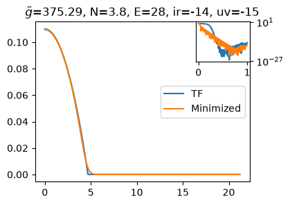
from gpe.Examples.tutorial import StateHOConvergence2
s0 = StateHOConvergence2(g=100, Lx=30.0, Nx=128, dmu=10.0)
axs = s0.plot(label="TF")
s = s0.get_initialized_state()
axs = s.plot(axs=axs, label="Minimized", plot_convergence=True)
axs[0].legend(loc='right');

[I 03:46:10 root] Patching zope.interface.document.asReStructuredText to format code
[I 03:46:10 numexpr.utils] NumExpr defaulting to 2 threads.

../_images/72f5d8240e016a4e1a01feeacab8ab9b2afa8f008099b46999a5cd53ea71bb7c.png

Our code solves the 2D GPE with

\[\begin{gather*} ( + g_{2D} \abs{\Phi}^2)\Phi = \mu \Phi\\ \phi = \frac{\Phi}{\sqrt{N}}\\ ( + g_{2D} N \abs{\phi}^2)\phi = \mu \phi\\ g_{2D} N = g n_1 \end{gather*}\]

Here we show the relative error between \(\mu(n_1)\) computed numerically and the formula above from the dr-GPE:

dmus = np.linspace(0.0001, 10.0, 100)
ss = [StateHOConvergence2(g=1, Lx=30.0, Nx=128, dmu=dmu).get_initialized_state()
      for dmu in dmus]
mus = np.array([s.get_mu() for s in ss])
Ns = np.array([s.get_N() for s in ss])
gtildes = np.array([s.get_gtilde() for s in ss])

g = 1.
n1s = s.g * Ns / g

s = ss[0]
a = 2
n1 = 1
hbar2_2m = s.hbar**2 / 2 / s.m
mw2_2 = s.m * s.w**2 / 2
gn1s = s.g * Ns
agn_4pi = a * gn1s / 4 / np.pi
sigma2 = np.sqrt((hbar2_2m + agn_4pi) / mw2_2)
mus_ = (hbar2_2m + agn_4pi)/sigma2 + mw2_2 * sigma2
fig, ax = plt.subplots()
ax.plot(n1s, mus/mus_ - 1)
ax.set(xlabel=r"$\mu_1$", ylabel=r"$\mu/\mu_{dr-GPE}-1$")
ax1 = plt.twinx()
ax1.plot(n1s, gtildes)

---------------------------------------------------------------------------
KeyboardInterrupt                         Traceback (most recent call last)
Cell In[3], line 2
dmus = np.linspace(0.0001, 10.0, 100)
----> 2 ss = [StateHOConvergence2(g=1, Lx=30.0, Nx=128, dmu=dmu).get_initialized_state()
     for dmu in dmus]
mus = np.array([s.get_mu() for s in ss])
Ns = np.array([s.get_N() for s in ss])

File ~/checkouts/readthedocs.org/user_builds/gpe/checkouts/latest/src/gpe/Examples/tutorial.py:155, in StateHOConvergence1.get_initialized_state(self, fix_N, minimize_kw)
m = MinimizeState(s0, fix_N=fix_N)
m.check()
--> 155 s1 = m.minimize(**minimize_kw)
s = self.copy()
s.set_psi(s1.get_psi())

File ~/checkouts/readthedocs.org/user_builds/gpe/checkouts/latest/src/gpe/minimize.py:751, in MinimizeState.minimize(self, psi_tol, E_tol, callback, _debug, **kw)
   return super().minimize(_debug=_debug, **kw)
else:
--> 751     x = super().minimize(**kw)
state = self.unpack(x)
if self.fix_N:

File ~/checkouts/readthedocs.org/user_builds/gpe/checkouts/latest/src/gpe/minimize.py:282, in Minimize.minimize(self, plot, callback, method, polish, broyden_alpha, broyden_opts, f_tol, x_tol, use_scipy, ignore_f, _test, _debug, _log, use_cache, bounds, **kw)
   if Version(sp.__version__) > Version("1.15.0"):
       options.pop("disp", None)
--> 282     res = self._minimize(
       f=_f,
       df=_df,
       x0=_x[0],
       method=method,
       callback=callback_,
       bounds=bounds,
       options=options,
   )
self.minimize_results = res
if not res.success:

File ~/checkouts/readthedocs.org/user_builds/gpe/checkouts/latest/src/gpe/minimize.py:311, in Minimize._minimize(self, f, df, x0, method, callback, bounds, options)
def _minimize(self, f, df, x0, method, callback, bounds, options):
   """Interface to the scipy minimizer."""
--> 311     res = sp.optimize.minimize(
       fun=f,
       jac=df,
       x0=x0,
       method=method,
       callback=callback,
       bounds=bounds,
       options=options,
   )
   res.f = f
   res.df = df

File ~/checkouts/readthedocs.org/user_builds/gpe/conda/latest/lib/python3.14/site-packages/scipy/optimize/_minimize.py:784, in minimize(fun, x0, args, method, jac, hess, hessp, bounds, constraints, tol, callback, options)
   res = _minimize_newtoncg(fun, x0, args, jac, hess, hessp, callback,
                            **options)
elif meth == 'l-bfgs-b':
--> 784     res = _minimize_lbfgsb(fun, x0, args, jac, bounds,
                          callback=callback, **options)
elif meth == 'tnc':
   res = _minimize_tnc(fun, x0, args, jac, bounds, callback=callback,
                       **options)

File ~/checkouts/readthedocs.org/user_builds/gpe/conda/latest/lib/python3.14/site-packages/scipy/optimize/_lbfgsb_py.py:461, in _minimize_lbfgsb(fun, x0, args, jac, bounds, disp, maxcor, ftol, gtol, eps, maxfun, maxiter, iprint, callback, maxls, finite_diff_rel_step, workers, **unknown_options)
g = g.astype(np.float64)
# x, f, g, wa, iwa, task, csave, lsave, isave, dsave = \
--> 461 _lbfgsb.setulb(m, x, low_bnd, upper_bnd, nbd, f, g, factr, pgtol, wa,
              iwa, task, lsave, isave, dsave, maxls, ln_task)
if task[0] == 3:
   # The minimization routine wants f and g at the current x.
   # Note that interruptions due to maxfun are postponed
   # until the completion of the current minimization iteration.
   # Overwrite f and g:
   f, g = func_and_grad(x)

KeyboardInterrupt: 

Non-Polynomial Schrödinger Equation (NPSEQ) in 1D (Tube)

Contents

Non-Polynomial Schrödinger Equation (NPSEQ) in 1D (Tube)#

Example: The Standard dr-GPE#