import mmf_setup; mmf_setup.nbinit()
import os
from pathlib import Path
FIG_DIR = Path(mmf_setup.ROOT) / '../Docs/_build/figures/'
os.makedirs(FIG_DIR, exist_ok=True)
import logging; logging.getLogger("matplotlib").setLevel(logging.CRITICAL)
%matplotlib
import numpy as np, matplotlib.pyplot as plt
try: from myst_nb import glue
except: glue = None
This cell adds /home/docs/checkouts/readthedocs.org/user_builds/gpe/checkouts/latest/src to your path, and contains some definitions for equations and some CSS for styling the notebook. If things look a bit strange, please try the following:
- Choose "Trust Notebook" from the "File" menu.
- Re-execute this cell.
- Reload the notebook.
Using matplotlib backend: module://matplotlib_inline.backend_inline
Effective Viscosity#
Here we consider viscous hydrodynamics in 1D of a fluid with number density \(n(x, t)\), velocity \(u(x, t)\), and energy density \(\mathcal{E}(n)\). Thermodynamics gives the “pressure” \(P(n)\) (just a force in 1D) as follows:
Here \(ϵ(n) = \mathcal{E}/n = E/N\) is the energy per particle, which sometimes appears. We will not use this here.
Conservation of particle number and momentum give the hydrodynamic equations:
where \(ν\) is a viscosity coefficient, and \(V(x, t)\) is an external potential.
A Comment on the Pressure
As discussed below, the momentum current is best expressed in terms of a pressure \(\mathcal{P}\). To do this, we are looking for a function \(\mathcal{P}\) whose gradient is \(n\) times the gradient of the potential
This contains both the intrinsic pressure \(P(n)\) from the equation of state of the fluid, and a contribution from the external potential \(F(x)\). The force \(F(x)\) here is the integrated force on the potential such that \(F(\infty)\) would be the force exerted by the fluid on the potential. I.e., if this potential were created by you sticking an object into the flow, then this would be the total force on the object. This is effectively a buoyant force but under appropriate boundary conditions – i.e. no potential drop – represents the drag force. This should not be confused with the local force \(-V_{,x}\) of the potential on the fluid.
It is a peculiarity of 1D that force and pressure have the same dimensions – more generally, one would obtain similar relationships after integrating a section.
Do It! Show that \((n\mathcal{E}'(n) - \mathcal{E})_{,x} = \bigl(\mathcal{E}'(n)\bigr)_{,x}\).
Just apply the chain rule and cancel terms
Unfortunately, since \(n(x)\) is a property of the solution, there is no simple way of expressing the force, so we cannot use this as a method of solution.
Interface with Vacuum
It is known (see e.g. [Lian et al., 2010] and references therein) that these equations, with a constant viscosity \(ν(n)\) leads to singular behavior at the interface with the vacuum (zero density). This can be alleviated by allowing \(ν(n)\) to depend on density. We do not consider the vacuum interface here, assuming that \(n>0\) everywhere in the problem domain.
A Physical Analogy: Shallow Water
To develop intuition, it is useful to have a familiar physical analogy. Consider an incompressible fluid of mass density \(\rho\) like water flowing along a channel of width \(w\) whose bottom height \(b(x)\) varies, but not enough to excite appreciable vertical dynamics. If the fluid height is \(\eta(x)\), then the internal energy density is given by the gravitational potential energy (here \(a_g\) is the acceleration due to gravity)
This suggests identifying the following 1D number density and coupling constant to match the GPE.
Comparison with Wikipedia
To compare with the conservative form of the shallow water equations, note that, in 2D, the following are equivalent, after application of the continuity equation:
Their form does not include the potential \(V(x)\) (they consider a flat bed). Explicitly
Conservation Laws#
Local conservation laws can be expressed in terms of a density \(a\) and a current \(c\) such that, under strict conservation, the integrated quantity \(A\) does not change with time:
The local expression of this conservation is
I.e. if the current vanishes far away, or if we work in a periodic box
Particle Number#
The first hydrodynamic equation demonstrates the conservation of particle number
This says that that total rate of change of particles in a region between \(x_L\) and \(x_R\) is equal to the flux of particles \(\Phi_{n}(x_L)\) entering the region from the left at \(x_L\) minus the flux of particles \(\Phi_{n}(x_R)\) leaving the region at \(x_R\) on the right. Notice that a positive flux corresponds to a flow to the right, consistent with the signs in this equation.
To Do. What is the meaning of \(D_t n = -nu_{,x}\)?
What is the physical meaning of the convective derivative of the density?
Why is this not zero?
Solution
The convective derivative characterizes how a quantity changes as you follow the particle flow. If you are following a particle, how does the density change? Well, this depends on how close the neighbouring particles are. The average distance to the neighbours changes iff there is a gradient in the velocity field. To see this, consider two particles at \(x_0 < x_1\) so that
I.e. the density only changes if the velocity of the relative particles is different – this is exactly what a gradient in the velocity indicates.
Momentum Density#
Multiply the continuity equation by \(u\) and add it to \(n\) times the Bernoulli equation:
Energy Density#
We can similarly consider the energy flux. The energy density is the sum of the kinetic, potential, and internal energies.
Here we see explicitly that energy conservation is violated by time-dependent potentials, and by a viscosity if the velocity field has a gradient \(u_{,x} \neq 0\). Thus, there will be no dissipation from this viscosity if we have simple sloshing in a harmonic trap where the velocity is constant. The second form shows explicitly that positive \(ν(n)\) will dissipate energy if \(\dot{V} = 0\) and also gives an energy density whose gradient is strictly decreasing for static solutions, which will be useful in our analysis below.
Numerical Checks
To make sure what we are doing makes sense, we give a concrete numerical example. We formulate the PDE as an ODE in time:
For details, see Viscosity Notes 1
Some Analytic Results for Static Flow#
For static problems, the current and momentum currents are constants everywhere:
Rankine-Hugoniot Conditions#
We start by considering solutions that are stationary far to the left \(j_L=u_Ln_L\) and far to the right \(j_R = u_Rn_R\) such that \(j_{,t} = (nu)_{,t} = 0\) and \(u_{,x} = 0\) in these asymptotic regions. The momentum conservation equation thus implies that \(mnu^2 +\mathcal{P}\) is constant in these regions, but the constant might differ on the left and right of some non-stationary region. Continuity implies that, if \(j_L \neq j_R\), then the transition region must move with velocity \(v\) to accommodate the change in particle number. This is one of the Rankine-Hugoniot conditions:
The usual application of this is to consider the motion of a shockwave or soliton which maintains its shape. Boosting to the co-moving frame, the problem becomes static everywhere and, in this frame, \(j_L = j_R = j\) is constant everywhere. Additionally, the momentum density is constant everywhere:
Considering again regions far from the potential where the flow is homogeneous, this implies that the total force on whatever potential exists in the intermediate region is
To be explicit, consider static flow: \(\dot{n} = \dot{u} = 0\) starting with constant density \(n_L\) and velocity \(u_L\) on the left with no potential \(V(x) = 0\):
From this, we can solve for the force:
If the flow far to the right or the potential is also constant \(u_{,x} \rightarrow 0\), then the total force on the potential is
If there is no potential \(V(x) = 0\), then \(F_{\text{total}} = 0\) and we find the Michelson–Rayleigh line:
(The final condition comes from energy conservation, but this is only independent if we consider finite temperature effects.)
Numerical Checks
To make sure what we are doing makes sense, we give a concrete example. To minimize the chance for error, we first implement the original equations in the form \(y=(n, ν(n)u, \bigl(ν(n)u\bigr)', F)\), looking for stationary solutions \(\dot{n} = \dot{u} = 0\). For an initial condition, we specify the density and velocity to the left of the barrier and directly integrate.
No Viscosity.#
In the limit of zero viscosity, particle number and energy conservation gives immediately
This directly relates the density to the potential and for \(j=0\), corresponds to the Thomas-Fermi (TF) approximation. For example, with the GPE \(\mathcal{E}'(n) = gn\), so
The second term corrects the TF density, and becomes significant at high rates of flow, or low densities. While the TF approximation gives some insight, the non-linear nature of the equation of state causes this to break down in an interesting way. This can be deduced from this expression: the correction term reduces the density, but this increases the significance of the correction. The feedback causes things to break earlier than expected.
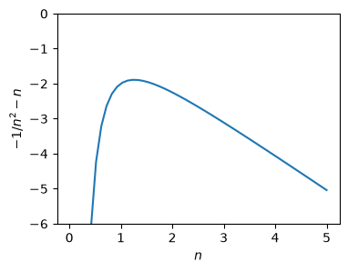
To see this, we consider this from a different perspective: as a limit on the maximum magnitude of the potential \(V(x)\) that will allow flow:
Maximizing the right-hand side for fixed \(E_0\) and \(j\), we find a critical density \(n_c\)
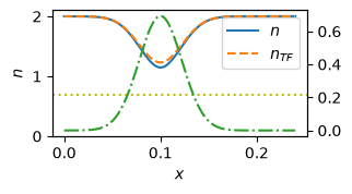
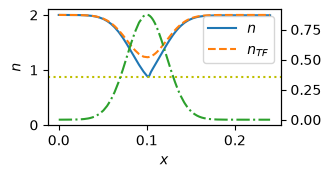
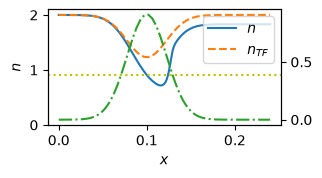
The velocity \(u_c\) associated with this critical density is the speed of sound \(c_s\) in the fluid at density \(n_c\). The interpretation of this was not obvious (at least to me) but very interesting (see the discussion below). For slow flow, \(u \ll u_c\), the TF approximation is valid, and if the potential is smooth, then the density will smoothly follow this \(n(x) \approx [\mu_0 - V(x)]/g\) in the GPE. For a barrier, the density always decreases, meaning that the velocity \(u = j/n\) increases. If one increases the current or increases the barrier height, however, then the fluid velocity over the barrier increases until it reaches the speed of sound \(u_c=c_s\). When this happens, \(n(x)\) – and consequently \(u(x)\) – develops a kink as the to independent solutions to the non-linear equation merge and vanish.
Important
We conclude that the static hydrodynamic equations cannot support hypersonic solutions – and if there is any viscosity, no matter how small, this cannot be neglected at the kink where \(u_{,xx}\) diverges!
This implies that the local velocity \(u\) can never exceed the local speed of sound implying a global critical density \(n_c\) which is related to the conserved current \(j\) by the non-linear equation
This in turn can be used to find the maximum allowable height of the potential supporting a given rate of flow (which depends on both \(j\) and \(n_0\)). Finite viscosity will affect these bounds in a non-trivial way.
What about the other direction? Suppose we have a barrier with maximum height \(V_{\max}\) and an initial density \(n_0\): what is the maximum flow \(j\) that can be supported?
Here, \(n_c\) depends on \(j\), giving a non-linear condition.
Nonlinearities.
When developing this, I ran into issues because of the nonlinear nature of the equations. I expected that the TF approximation would break down when
was such that the second term started to become significant. The equations broke down, however, well before this, developing a kink with a sharp drop in density for significantly lower \(V_0\) than expected. The reason turns out to be related to the non-linear nature of the solution.
Starting with the GPE, we have a cubic:
The problem is that the relevant solution becomes degenerate (and then vanishes) when \(P_n'(n) = 0\) at the root
This gives a constraint on \(V\) to prevent the development of a kink in the density:
Generalizing, we consider the function
and solve for \(P(n_c) = P'(n_c) = 0\):
This defines a critical flow velocity \(u_c\) which is the speed of sound \(c_s\) in the fluid:
Flow Past a Barrier#
It is interesting to consider flow past a weak barrier. In the shallow-water hydrodynamic picture, this is what happens when a river flows past a weir. When water flows from a slow-moving river over a weir, a thin layer of water moves rapidly over the weir as required by continuity. From this intuition, we might expect the density \(n\) over the barrier to decrease as the velocity \(u\) increases keeping \(j=un\) constant.
This intuition is in contrast with the picture of free particles, which lose speed as they move up and over the potential, gaining potential energy as they lose kinetic energy. In this case, continuity requires that the density increase, in contrast with the typical behavior of a weir. This conflict suggests a transition between a hydrodynamic regime where interactions dominate (weir) and a ballistic or kinetic regime where kinetic energy dominates, however, as discussed above, this ballistic regime cannot be realized in the static problem as it requires hypersonic flow.
We thus limit our analysis here to subsonic flow, asking, what force does a fluid with viscosity exert as it flows over a barrier. The density and momentum continuity equations give the following in terms of the constants \(j\) and \(p\):
We assume that, far from the potential, \(u_{,x} = 0\) so we can drop the viscosity term in this equation. The net force due to the potential is thus
GPE
Specifically, for the GPE, we have
From this we see several features:
If we have no flow \(j=0\), then there is a force in the direction of the lower density. This makes sense: we have a dam between two reservoirs, and the higher pressure wins.
If there is flow, then the force decreases in magnitude until, at a critical current, the direction of the force reverses.
There is no force on the potential if \(n_L = n_R\), regardless of the flow velocity.
Can we independently adjust \(n_L\), \(n_R\), and \(j\)? This is not obvious. We can certainly start with \(n_L = n_R\) and an arbitrary \(j\) if we have no barrier.
We can also consider the energy density
Dimensional Analysis#
We start with a naïve dimensional analysis of the 1D problem in the GPE with water flowing over a weir of height \(V_0\), width \(\sigma\), and potential drop \(\delta\). Here we consider steady state flow with (conserved) current \(j\) and initial density \(n_L = n_0\).
From these, we can choose three independent quantities to set our units. We start with \(m = n_0 = j = 1\):
This gives the following dimensionless quantities
About Naïve Dimensional Analysis
Since \(m\) is intrinsic to the problem, and \(j\) is conserved, we are pretty sure that these are good parameter choices. However, without further analysis, it is not clear which of the other parameters will be of most relevance for an analysis. For example, instead of \(g\), the speed of sound might be relevant, but should one use the density \(n_0\) or the minimum density at the top of the barrier? Most likely, the parameters discussed above in section No Viscosity. will play an important role, but we need to start somewhere, so we start here.
We would also like to vary the viscosity \(ν\), so we want to keep it as a parameter. Similarly with \(V_0\) and \(\sigma\). Finally, we have \(g\), but it might be reasonable to vary this, so we choose to fix our units with \(j\), \(n_0\), and \(m\).
Later refinements might include setting \(2m = 1\) so that \(\tilde{V}_0 = 1\) corresponds to particles with just enough kinetic energy to overcome the barrier. A better parameterization might include the effects of pressure.
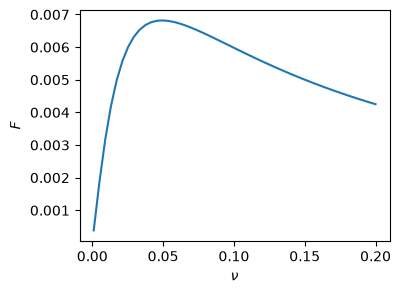
To simplify our analysis, we start by considering the limit of a step-potential: \(\sigma \rightarrow 0\) and \(V_0 = 0\), reducing our exploration to a 3-dimensional parameter space characterized by the viscosity \(ν\), interactions \(g\) (compressibility), and step size \(\delta\).
nus = np.linspace(0.001, 0.2)
fs = []
Fs = []
for nu in nus:
f = Flow1(n0=2.0, v0=1.0, V0=0.1, nu=nu)
res = f.solve(x_L=5.0, atol=1e-12, rtol=1e-12)
fs.append(f)
Fs.append(res.F[-1]-res.F[0])
fig, ax = plt.subplots(1, 1, figsize=(4,3))
ax.plot(nus, Fs)
ax.set(xlabel=r"$ν$", ylabel="$F$")
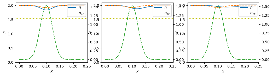
ind = np.argmax(Fs)
fig, axs = plt.subplots(1, 3, figsize=(12, 3))
for f, ax in zip([fs[0], fs[ind], fs[-1]], axs):
f.plot(ax=ax)
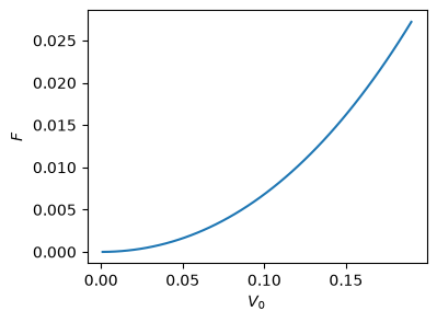
nu = 0.05
V0s = np.linspace(0.001, 0.19)
fs = []
Fs = []
for V0 in V0s:
f = Flow1(n0=2.0, v0=1.0, V0=V0, nu=nu)
res = f.solve(x_L=5.0, atol=1e-12, rtol=1e-12)
fs.append(f)
Fs.append(res.F[-1]-res.F[0])
fig, ax = plt.subplots(1, 1, figsize=(4,3))
ax.plot(V0s, Fs)
ax.set(xlabel=r"$V_0$", ylabel="$F$")
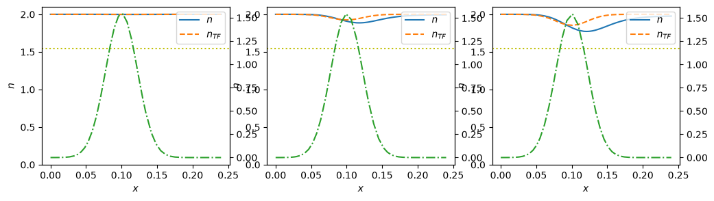
ind = len(V0s)//2
fig, axs = plt.subplots(1, 3, figsize=(12, 3))
for f, ax in zip([fs[0], fs[ind], fs[-1]], axs):
f.plot(ax=ax)
Misc. Work (Incomplete)
The density and momentum continuity equations give the following in terms of the constants \(j\) and \(p\):
Far from the potential, \(u_{,x} = 0\) so we can drop the viscosity term. The net force due to the potential is thus
Specifically, for the GPE, we have
If we have no flow \(j=0\), then this tells us that there is a force in the direction of the lower density, but this decreases in magnitude as a velocity flows, until at a critical current, the direction increases.
Consider a step-like potential with small \(\epsilon\rightarrow 0\):
Working backwards, let \(u(x)\) be linear in the region \([0, \epsilon]\)
In this interval, we have
For \(x \gg \epsilon\) we have
where
For small \(\delta n\) we can write
which is exact for the GPE \(P(n) = gn^2/2\). This gives:
This can be iterated a couple of times to converge. If \(\delta n\) is small, we can expand:
Let’s start with a perfect fluid without viscosity \(ν=0\) flowing over a step The momentum continuity equation gives
Starting with \(n(x<0) = n_L\), \(u(x<0) = u_L\), and \(F(x<0) = 0\) with \(j=u_Ln_L\) constant, we have
Integrating the momentum conservation equation across the potential we have:
A Numerical Example: Steady-State Flow#
We start with steady-state flow over a barrier. To make sure what we are doing makes sense, we give a concrete example. To minimize the chance for error, we first implement the original equations in the form \(y=(n, u, u', F)\), looking for stationary solutions \(\dot{n} = \dot{u} = 0\). For an initial condition, we specify the density and velocity to the left of the barrier and directly integrate.
These equations are not very easy to reason with, however: e.g., they look singular in the limit of vanishing viscosity. To deal with this, we replace the velocity with a variable \(q = ν u_{,x}\), and use the continuity equation to remove the velocity dependence:
Instead, we use the continuity \(j=nu\) and positivity of \(n\) which suggest introducing the variable \(q = \ln n\):
# Check some of the formulae
f = Flow()
res = f.solve(atol=1e-10, rtol=1e-10)

m, j, nL, nu = f.m, f.n0*f.v0, f.n0, f.nu

# Continuity
assert np.allclose(j, res.n*res.u)

# Force
P, PL = map(f.get_P, [res.n, nL])
x, V = res.x, f._V(res.x)
dE, dEL, ddE = f.get_Eint(res.n, d=1), f.get_Eint(nL, d=1), f.get_Eint(res.n, d=2)
F1 = m*j**2 * (1/nL - 1/res.n) + PL - P + m*nu*res.du
assert np.allclose(res.F, F1, atol=1e-7)

# This has some numerical artefacts at the kinks.  We smooth these:
res.j = res.u*res.n
e = (m*res.j*res.u**2/2 + res.j*(V + dE) - m*nu*res.u*res.du)
de = sp.interpolate.UnivariateSpline(x, e, s=1e-13).derivative()(x)
assert np.allclose(de, -m*nu*res.du**2, atol=3e-4)
Details.
The original equations should be solved to isolate \(n_{,x}\) and \(u_{,x}\):
Dividing by \(n\) and \(u\), we obtain
This follows from the continuity equation which directly implies
Removing the Velocity
Alternatively, we can use the conservation equation to remove the velocity from our equations since \(nu = n_0u_0 = j_0 = \text{const.}\) everywhere:
The momentum current is
We will use the GPE equation of state:
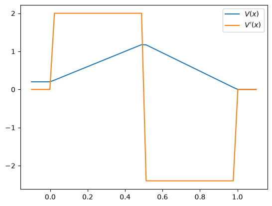
and a piecewise linear potential with height \(V_0\), width \(L\), and potential difference \(\delta V\) dropping from left to right.
This gives us the following intrinsic parameters
In addition, we have the extrinsic parameters related to the initial state
We now choose three constants to define the units of mass, distance, and time. Without performing a full analysis, it is hard to tell what will ultimately be most appropriate, so we start with an educated guess. The mass scale is naturally set by \(m=1\).
Some other quantities of relevance include the speed of sound \(c_s = \sqrt{gn_0/m}\) and the conserved current \(j = n_0u_0\), \([j] = 1/T\). More complicated parameters might be the minimum speed required to overcome the barrier.
To start, we will focus on the initial state
Analysis
In the previous plot, we look at static flow across a barrier as a function of the flow-rate (current) \(j\). We plot the total force on the barrier (solid), and the density drop (dashed).
We start with the two conservation laws for density and momentum far to the left and right of the potential, assuming that \(u_{,x}=0\) in these regions, and setting \(F(x_L) = 0\) and \(F(x_R) = F\):
Assuming that \(u_{,x} = 0\) far from the potential (static flow), and setiing \(V(x_R) = 0\), we have the following after integrating the energy current:
Correction Needed Below
The following analysis is incorrect. It is missing the factor of \(1/n\) discussed above, and neglects to include a difference in the potential from one side to the other (DC offset) required to maintain a persistent flow in the presence of dissipation.
Steady State (Incorrect)
Now consider steady-state flow \(n(x, t) = n(x)\), \(u(x, t) = u(x)\). These become:
The first equation establishes that the flux \(Φ = nu\) is the same at every point, allowing us to exchange velocity \(u\) for density \(n\):
Let’s assume that \(V(x)\) has compact support over \([0, L]\), then we can give boundary conditions \(u(0) = u_0\), \(u_{,x}(0) = 0\). The second equation and be integrated once to give the non-linear first-order equation
For general \(V(x)\), this has no analytic solution, but we can compute a perturbative solution if we let \(V(x) \rightarrow \lambda V(x)\) where \(\lambda \ll 1\). We note that \(u(x) = u_0\) is a solution for \(\lambda = 0\) and write $\(u(x) = u_0 + \lambda u_1(x) + \lambda^2 u_2(x) + O(\lambda^3).\)\(_Note: In what follows, we revert back to the notation_ \)u_1’ = [u_1]{,x}$…
I originally wrote it this way, and have not changed it yet._
As shown below, we originally tried expanding to first order in \(\lambda\), but found this was insufficient, so we expand to second order in \(\lambda\) obtaining the following linear equations for \(u_1\) and \(u_2\):
where we have introduced the constants
Do it!
To solve this problem, one needs to find a solution to the following inhomogeneous differential equation:
where \(a>0\). We are particularly interested in the limit where \(a\rightarrow 0\), which will correspond to zero viscosity.
You should find that
Notice that this has a non-analytic dependence \(e^{x/a}\) on the parameter \(a \propto ν\). Show that, when expanding from the appropriate limit, all coefficients of the Taylor series for \(e^{x/a}\) in powers of \(a\) are zero. This makes it somewhat tricky to expand for small viscosities since all terms with such a factor will vanish.
Argue, however, that there may be an analytic particular solution \(u_1(x, a)\) whose form can be found by expanding in powers of \(a\). We can then write the general solution as
The non-analytic piece, thus describes transients (exponentially decaying in the appropriate direction) induced by the initial (boundary) conditions.
Show that this particular solution is:
For example, this allows us to easily solve for \(f(x) = \sin(kx)\):
We can easily check by differentiating that this satisfies the original equation.
Force
The (buoyant) force acting on the potential \(V(x)\) is
Returning to our original equation, we have
A Numerical Example
To make sure what we are doing makes sense, we give a concrete example. To minimize the chance for error, we implement the original equations in the form \(y=(n, u, u', F)\), allowing for a density-dependent viscosity:
Notice that the potential causes the density to change, then the viscosity allows this to relax outside of the shaded region where the potential is active. We now check some relationships.
Now let’s check the small \(λ\) approximations:
The following code demonstrates that the order \(λ\) solution \(u_1(x)\) gives the correct force when integrated. (There is no need to compute \(u_2(x)\).)
Thus, the complete solution to order \(λ\) is to solve the following problem:
Note that the coefficient \(c\) here is generally less than zero. We can see this by noting that the speed of sound in a material is \(c_s\) is:
Thus, for subsonic flow \(u_0<c_s\), \(c<0\). We keep this sign convention to avoid many other signs below. The homogeneous solution is \(u_1(x) = Ae^{cx}\). To find the general solution, there are several options:
One is the method of variation of parameters can be used, promoting \(A → A(x)\) to find
\[\begin{gather*} u_1(x) = A(x)e^{cx}, \qquad A'(x) e^{cx} = V(x)/{mν}, \qquad A(x) = \frac{1}{mν}\int_0^xd{y}\; e^{-cy}V(y), \\ u_1(x) = \frac{1}{mν}\int_0^xd{y}\; e^{c(x-y)}V(y),\\ F = \frac{-λ^2n_0}{mu_0}\int_{0}^{L}d{x}\;\int_0^xd{y}\; e^{c(x-y)}V(y)V'(x). \end{gather*}\]The integral is over the lower triangle \(y<x\) of the box \((x, y) ∈[0, L]×[0,L]\). To better express the dimensionality of the solution, we write the potential as \(V(x) = V_0U(x/L)\) so that the shape is described by the dimensionless function \(U(\xi)\), and we introduce the dimensionless quantity \(\kappa \propto \nu\):
\[\begin{gather*} λV(x) = λV_0U(x/L), \qquad \kappa = \frac{1}{-cL} = \frac{\nu}{-aL},\\ \begin{aligned} F &= \frac{-λ^2n_0V_0^2L}{mu_0} \underbrace{\int_{0}^{1}d{x}\;\int_0^xd{y}\; e^{(y-x)/\kappa}U(y)U'(x)}_{-\kappa^2 f(\kappa, U)},\\ &= \frac{Lu_0\kappa^2}{\nu}\frac{λ^2V_0^2n_0}{mu_0^2}f(\kappa, U). \end{aligned} \end{gather*}\]While formally correct, this solution obscures the viscosity dependence. We will see below that the normalization chosen here for \(f(\kappa, U)\) makes sense in the limit of small viscosity:
\[\begin{gather*} f(\kappa, U) = -\int_{0}^{1}d{x}\;\int_0^xd{y}\; \frac{e^{(y-x)/\kappa}}{\kappa^2}U(y)U'(x) \end{gather*}\]Another is formal manipulation. We first introduce the parameter \(a=cν\) which is independent of the viscosity, then solve algebraically treating the derivative operator as a matrix:
\[\begin{align*} νu_1'(x) &= au_1(x) + V(x)/m, \\ u_1(x) &= \frac{1}{\left(1-\frac{ν}{a}\frac{d}{d{x}}\right)}\frac{-V(x)}{am},\\ &= -\frac{V(x)}{am} - \frac{νV'(x)}{a^2m} - \frac{ν^2V''(x)}{a^3m} + O(ν^3). \end{align*}\]This is nice because it immediately allows us to expand in powers of \(ν\) by expanding \(1/(1-x) =1+x+x^2+x^3+\cdots\):
\[\begin{gather*} F = \frac{λ^2n_0 V_0^2}{mau_0} \int_{0}^{1}d{x}\;\left( U(x)U'(x) - \kappa[U'(x)]^2 + \kappa^2U''(x)U'(x) + O(ν^3) \right) \end{gather*}\]Since \(U(0)=U(1)=0\), the first term, which is a total derivative \((U^2)'/2\), vanishes. This gives:
\[\begin{align*} F &= \frac{mλ^2n_0}{au_0}\frac{V_0^2}{m^2}(-\kappa)\overbrace{ \Biggl( \int_{0}^{1}d{x}\;[U'(x)]^2 -\kappa\left.\frac{[U'(x)]^2}{2}\right|_{0}^{1} +\kappa^2\int_{0}^{1}d{x}\;U'(x)U'''(x) + O(ν^3) \Biggr)}^{f(\kappa, U)}\\ &= \frac{mλ^2n_0}{au_0}\frac{ν}{a} \frac{V_0^2}{m^2L} f(\kappa, U). \end{align*}\]This justifies the form of \(f(\kappa, U)\) chosen above. If we choose a symmetric potential so that \(|U'(0)| = |U'(1)|\), then the second term vanishes, allowing us to precisely define what a small viscosity means:
\[\begin{gather*} \frac{ν^2}{a^2} \frac{\int_{0}^{L}d{x}\;V'(x)V'''(x)} {\int_{0}^{L}d{x}\;[V'(x)]^2} = \kappa^2 \frac{\int_{0}^{1}d{x}\;U'(x)U'''(x)} {\int_{0}^{1}d{x}\;[U'(x)]^2} \ll 1. \end{gather*}\]
We now replace the parameter \(a\) with the speed of sound \(c_s\). The final result, to leading order in \(λ\) is:
Here we have expressed the results in terms of the dimensionless Reynold’s number \(\mathrm{Re}\) and the ratio of the speed of sound \(c_s\) to the flow \(u_0\). Note that the force diverges as the flow speed approaches the speed of sound. The dependence on the shape appears with the dimensionless parameter \(\kappa = ν/(-aL)\):
Caution: The expansion in \(\kappa \propto \nu\) here justifies our choice for the form of \(f(\kappa, U)\) and the corresponding separation of dimensionful parameters, but it turns out that this series does not converge to the solution. We now demonstrate this. Consider for example, the dimensionless potential
This solution contains the non-analytic term \(e^{-1/\kappa}\) whose Taylor series for positive \(\kappa\) is zero. Thus, the series expansion converges to the incorrect form of:
fails to converge.
This figure shows that the integral gives the correct formula, and that for large \(\kappa\) the non-analytic piece is correct. It also shows that we have made a mistake in our series approximation. Please fix!
Here is \(U(x) = \sin^2\bigl(\pi(x-1)\bigr)\):
If we choose \(U(\xi) = U(1-\xi)\) to be symmetric, then the even terms vanish, and we can write:
Here are a couple of special cases. Note: For numerical work, it might be better to use a potential that is sufficiently flat at the boundaries, hence the higher power. This is what I have used in the code. (Please check these.)
Thus, for a sinusoidal potential (please check):
These can also be obtained by :
(I found these from the expansion https://oeis.org/A092812):
>>>>>>> variant B
---
jupytext:
  cell_metadata_filter: -all
  formats: md:myst,ipynb
  main_language: python
  text_representation:
    extension: .md
    format_name: myst
    format_version: 0.13
    jupytext_version: 1.13.7
kernelspec:
  display_name: Python 3 (ipykernel)
  language: python
  name: python3
---

```{code-cell}
import mmf_setup; mmf_setup.nbinit()
import os
from pathlib import Path
FIG_DIR = Path(mmf_setup.ROOT) / '../Docs/_build/figures/'
os.makedirs(FIG_DIR, exist_ok=True)
import logging; logging.getLogger("matplotlib").setLevel(logging.CRITICAL)
%matplotlib inline
import numpy as np, matplotlib.pyplot as plt
try: from myst_nb import glue
except: glue = None
Effective Viscosity (Old)
Conservation Laws
Particle Number
The first hydrodynamic equation demonstrates the conservation of particle number
This says that that total rate of change of particles in a region between \(x_L\) and \(x_R\) is equal to the flux of particles \(\Phi_{n}(x_L)\) entering the region from the left at \(x_L\) minus the flux of particles \(\Phi_{n}(x_R)\) leaving the region at \(x_R\) on the right. Notice that a positive flux corresponds to a flow to the right, consistent with the signs in this equation.
To Do. What is the meaning of \(D_t n = -nu_{,x}\)?
What is the physical meaning of the convective derivative of the density?
Why is this not zero?
Solution
The convective derivative characterizes how a quantity changes as you follow the particle flow. If you are following a particle, how does the density change? Well, this depends on how close the neighbouring particles are. The average distance to the neighbours changes iff there is a gradient in the velocity field. To see this, consider two particles at \(x_0 < x_1\) so that
I.e. the density only changes if the velocity of the relative particles is different – this is exactly what a gradient in the velocity indicates.
Momentum Density#
Multiply the continuity equation by \(u\) and add it to \(n\) times the Bernoulli equation:
This means that, if we have a static solution, then the following is constant everywhere:
Unfortunately, as mentioned above, the force depends on the solution through the density, so we can use this to check and interpret results, but it does not help us solve anything.
Energy#
We can similarly consider the energy flux. The energy density is the sum of the kinetic, potential, and internal energies.
Here we see explicitly that energy conservation is violated by time-dependent potentials, and by a viscosity if the velocity field has a gradient \(u_{,x} \neq 0\). Thus, there will be no dissipation from this viscosity if we have simple sloshing in a harmonic trap where the velocity is constant. The second form gives a current density whose gradient is strictly decreasing if viscosity is active and \(\dot{V}=0\).
An Analytic Example#
Consider static flow: \(\dot{n} = \dot{u} = 0\). The density and momentum continuity equations give the following in terms of the constants \(j\) and \(p\):
Consider a step-like potential with small \(\epsilon\rightarrow 0\):
Working backwards, let \(u(x)\) be linear in the region \([0, \epsilon]\)
In this interval, we have
For \(x \gg \epsilon\) we have
where
For small \(\delta n\) we can write
which is exact for the GPE \(P(n) = gn^2/2\). This gives:
This can be iterated a couple of times to converge. If \(\delta n\) is small, we can expand:
Let’s start with a perfect fluid without viscosity \(\nu=0\) flowing over a step The momentum continuity equation gives
Starting with \(n(x<0) = n_L\), \(u(x<0) = u_L\), and \(F(x<0) = 0\) with \(j=u_Ln_L\) constant, we have
Integrating the momentum conservation equation across the potential we have:
A Numerical Example: Steady-State Flow#
We start with steady-state flow over a barrier. To make sure what we are doing makes sense, we give a concrete example. To minimize the chance for error, we implement the original equations in the form \(y=(n, u, u', F)\), looking for stationary solutions \(\dot{n} = \dot{u} = 0\):
Removing the Velocity
Alternatively, we can use the conservation equation to remove the velocity from our equations since \(nu = n_0u_0 = j_0 = \text{const.}\) everywhere:
The momentum current is
We will use the GPE equation of state:
and a piecewise linear potential.
import scipy as sp
x = np.linspace(-0.1, 1.1)
V0 = 1.2
dV = 0.2
xp, fp = [0, 0.5, 1.0], [dV, V0, 0]
V = sp.interpolate.InterpolatedUnivariateSpline(xp, fp, k=1, ext='const')
plt.plot(x, V(x), label='$V(x)$')
plt.plot(x, V.derivative()(x), label="$V'(x)$")
plt.legend()
<matplotlib.legend.Legend at 0x757e348bc980>
from scipy.integrate import solve_ivp
import scipy as sp

class Flow:
    m = 1.0
    g = 1.0
    nu = 0.1  # Viscosity
    V0 = 0.2  # Potential barrier height
    L = 0.2   # Length of barrier

    n0 = 1.0  # Steady-state density on the left.
    v0 = 0.1  # Steady-state velocity on the left.
    dV = 0.1  # Potential drop (magnitude)

    # Boundary conditions on the left
    def __init__(self, **kw):
        for key in kw:
            if not hasattr(self, key):
                raise ValueError(f"Unknown {key=}")
            setattr(self, key, kw[key])
        self.init()

    def init(self):
        xp, fp = [0, self.L/2, self.L], [self.dV, self.V0, 0]
        self._V = sp.interpolate.InterpolatedUnivariateSpline(xp, fp, k=1, ext='const')
        self._dV = self._V.derivative()

    def get_Eint(self, n, d=0):
        if d == 0:
            return self.g * n**2 /2
        elif d == 1:
            return self.g * n
        elif d == 2:
            return self.g
        else:
            return 0

    def compute_dy_dx(self, x, y):
        n, u, du, F = y
        dn = -n*du/u
        ddu = n * (u*du + (self._dV(x) + self.get_Eint(n, d=2)*dn)/self.m) / self.nu
        dF = n * self._dV(x)
        return (dn, du, ddu, dF)

    def solve(self, dv0=0.0, x0_L=-0.1, x_L=2.0):
        x_span = (x0_L*self.L, x_L*self.L)
        y0 = (self.n0, self.v0, dv0, 0.0)
        res = solve_ivp(self.compute_dy_dx,  y0=y0, t_span=x_span, max_step=0.001)
        assert(res.success)
        res.x = res.t
        res.n, res.v, res.dv, res.F = res.y
        res.dn, dv, res.ddv, res.dF = self.compute_dy_dx(res.x, res.y)
        self.res = res
        return res

f = Flow()
res = f.solve()
Analysis#
We start with the two conservation laws for density and momentum far to the left and right of the potential, assuming that \(u_{,x}=0\) in these regions, and setting \(F(x_L) = 0\) and \(F(x_R) = F\):
Assuming that \(u_{,x} = 0\) far from the potential (static flow), and setiing \(V(x_R) = 0\), we have the following after integrating the energy current:
Correction Needed Below#
The following analysis is incorrect. It is missing the factor of \(1/n\) discussed above, and neglects to include a difference in the potential from one side to the other (DC offset) required to maintain a persistent flow in the presence of dissipation.
Steady State (Incorrect)#
Now consider steady-state flow \(n(x, t) = n(x)\), \(u(x, t) = u(x)\). These become:
The first equation establishes that the flux \(Φ = nu\) is the same at every point, allowing us to exchange velocity \(u\) for density \(n\):
Let’s assume that \(V(x)\) has compact support over \([0, L]\), then we can give boundary conditions \(u(0) = u_0\), \(u_{,x}(0) = 0\). The second equation and be integrated once to give the non-linear first-order equation
For general \(V(x)\), this has no analytic solution, but we can compute a perturbative solution if we let \(V(x) \rightarrow \lambda V(x)\) where \(\lambda \ll 1\). We note that \(u(x) = u_0\) is a solution for \(\lambda = 0\) and write $\(u(x) = u_0 + \lambda u_1(x) + \lambda^2 u_2(x) + O(\lambda^3).\)\(_Note: In what follows, we revert back to the notation_ \)u_1’ = [u_1]{,x}$…
I originally wrote it this way, and have not changed it yet._
As shown below, we originally tried expanding to first order in \(\lambda\), but found this was insufficient, so we expand to second order in \(\lambda\) obtaining the following linear equations for \(u_1\) and \(u_2\):
where we have introduced the constants
Do it!#
To solve this problem, one needs to find a solution to the following inhomogeneous differential equation:
where \(a>0\). We are particularly interested in the limit where \(a\rightarrow 0\), which will correspond to zero viscosity.
You should find that
Notice that this has a non-analytic dependence \(e^{x/a}\) on the parameter \(a \propto ν\). Show that, when expanding from the appropriate limit, all coefficients of the Taylor series for \(e^{x/a}\) in powers of \(a\) are zero. This makes it somewhat tricky to expand for small viscosities since all terms with such a factor will vanish.
Argue, however, that there may be an analytic particular solution \(u_1(x, a)\) whose form can be found by expanding in powers of \(a\). We can then write the general solution as
The non-analytic piece, thus describes transients (exponentially decaying in the appropriate direction) induced by the initial (boundary) conditions.
Show that this particular solution is:
For example, this allows us to easily solve for \(f(x) = \sin(kx)\):
We can easily check by differentiating that this satisfies the original equation.
Force#
The (buoyant) force acting on the potential \(V(x)\) is
Returning to our original equation, we have
A Numerical Example#
To make sure what we are doing makes sense, we give a concrete example. To minimize the chance for error, we implement the original equations in the form \(y=(n, u, u', F)\), allowing for a density-dependent viscosity:
%matplotlib inline
import matplotlib
from functools import partial
import numpy as np, matplotlib.pyplot as plt
from scipy.integrate import solve_ivp
matplotlib.rcParams['figure.figsize'] = (4,3)

m = 1.8
nu0 = 0.032
L = 1.3
n0 = 0.85
u0 = 0.773/2
Φ = n0*u0
g_m = 1.5
lam = 0.02

def mu(n, d=0):
    """Return the GPE chemical potential derivatives."""
    if d == 0:
        return m*g_m*n
    elif d == 1:
        return m*g_m+0*n
    elif d == 2:
        return 0*n

def mu(n, d=0):
    """Return the UFG chemical potential derivatives."""
    if d == 0:
        return m*g_m*n**(5/3)
    elif d == 1:
        return 5/3*m*g_m*n**(2/3)
    elif d == 2:
        return 10/9*m*g_m*n**(-1/3)

def mu_(n, d=0):
    """Return the GPE chemical potential derivatives."""
    if d == 0:
        return m*g_m*n**3
    elif d == 1:
        return 3*m*g_m*n**2
    elif d == 2:
        return 6*m*g_m*n

def V(x, d=0):
    """Return the external potential or derivative."""
    if d == 0:
        return np.where(abs(2*x/L-1) < 1, m*x*(x-L), 0)
    elif d == 1:
        return np.where(abs(2*x/L-1) < 1, m*(2*x-L), 0)
    elif d == 2:
        return np.where(abs(2*x/L-1) < 1, m*2, 0)

def V(x, d=0):
    """Return the external potential or derivative."""
    if d == 0:
        return np.where(abs(2*x/L-1) < 1,
        m*np.sin(np.pi*(x-L)/L)**2, 0)
    elif d == 1:
        return np.where(abs(2*x/L-1) < 1,
        np.pi/L*m*np.sin(2*np.pi*(x-L)/L), 0)
    elif d == 2:
        return np.where(abs(2*x/L-1) < 1,
        2*np.pi**2/L**2*m*np.cos(2*np.pi*(x-L)/L), 0)
    elif d == 3:
        return np.where(abs(2*x/L-1) < 1,
        -4*np.pi**3/L**3*m*np.sin(2*np.pi*(x-L)/L), 0)

def V(x, d=0):
    """Return the external potential or derivative."""
    s = np.sin(np.pi*(x-L)/L)
    ds = np.cos(np.pi*(x-L)/L)*np.pi/L
    ds2 = -np.sin(np.pi*(x-L)/L)*(np.pi/L)**2
    ds3 = -np.cos(np.pi*(x-L)/L)*(np.pi/L)**3

    if d == 0:
        return np.where(abs(2*x/L-1) < 1,
        m*s**4, 0)
    elif d == 1:
        return np.where(abs(2*x/L-1) < 1,
        m*4*s**3*ds, 0)
    elif d == 2:
        return np.where(abs(2*x/L-1) < 1,
        m*(12*s**2*ds**2 + 4*s**3*ds2), 0)
    elif d == 3:
        return np.where(abs(2*x/L-1) < 1,
        m*(24*s*ds**3 + 36*s**2*ds*ds2 + 4*s**3*ds3), 0)


def nu(n, nu0=1.0, gamma=0.0, d=0):
    """Return the density-dependent viscosity."""
    if d == 0:
        return nu0*n**gamma
    elif d == 1:
        return nu0*gamma*n**(gamma-1)

def compute_dy_dt(x, y, lam=lam, nu0=nu0,
                  u0=u0, n0=n0, m=m):
    n, u, du, F = y
    dn = -n*du/u
    dV = lam*V(x, d=1)
    #ddu = (m*u*du + dV + mu(n, d=1)*dn)/m/nu
    nu_, dnu_ = [nu(n, nu0=nu0, d=d) for d in [0, 1]]
    ddu = (n*(m*u*du + dV + mu(n, d=1)*dn)/m - du*dnu_*dn)/nu_
    dF = n*dV
    return (dn, du, ddu, dF)

y0 = (n0, u0, 0, 0)

res = solve_ivp(
    partial(compute_dy_dt, nu0=0.2, lam=0.5),
    y0=y0,
    t_span=(-L, 5*L), max_step=0.001)
x = res.t
n, u, du, F = res.y
assert np.allclose(n*u, n0*u0)
fig, ax = plt.subplots()
ax.plot(x/L, n/n0, label="$n$")
ax.plot(x/L, u/u0, label="$u$")
ax.axvspan(0, 1, color='y', alpha=0.5)
ax.set(xlabel="$x/L$", ylabel="$n/n_0$", title=f"{n[0]=}, {n[-1]=}", );
plt.legend(loc="upper left")
ax = plt.twinx()
ax.plot(x/L, F, '--C1', label="$F$")
ax.legend(loc="lower right")
ax.set(ylabel="$F$");
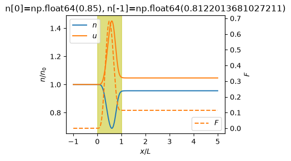
Notice that the potential causes the density to change, then the viscosity allows this to relax outside of the shaded region where the potential is active. We now check some relationships.
# Check that the potential and mu derivatives are correct
fig, axs = plt.subplots(1, 2)
ax = axs[0]
ax.plot(x/L, V(x), 'C0')
ax.plot(x/L, V(x, d=1), 'C1-')
ax.plot(x/L, np.gradient(V(x), x), 'C1:')
ax.plot(x/L, V(x, d=2), 'C2-')
ax.plot(x/L, np.gradient(V(x, d=1), x), 'C2:')
ax.plot(x/L, V(x, d=3), 'C3-')
ylim = ax.get_ylim()
ax.plot(x/L, np.gradient(V(x, d=2), x), 'C3:')
ax.set(ylim=ylim)

ax = axs[1]
ns = np.linspace(n0/2, 2*n0)
ax.plot(ns/n0, mu(ns), 'C0')
ax.plot(ns/n0, mu(ns, d=1), 'C1-')
ax.plot(ns/n0, np.gradient(mu(ns), ns), 'C1:')
ax.plot(ns/n0, mu(ns, d=2), 'C2-')
ax.plot(ns/n0, np.gradient(mu(ns, d=1), ns), 'C2:')
[<matplotlib.lines.Line2D at 0x757e34547a10>]
from functools import partial

def get_F(lam=lam, nu=nu, u0=u0, n0=n0, m=m, L=L, tol=1e-7):
    y0 = (n0, u0, 0, 0)
    dy_dt = partial(compute_dy_dt, lam=lam, nu=nu,
                    u0=u0, n0=n0, m=m)
    res = solve_ivp(dy_dt,
                    y0=y0, t_span=(0, L),
                    method='BDF',
                    rtol=tol, atol=tol)
    x = res.t
    n, u, du, F = res.y
    return F[-1]

lams = np.linspace(0, 0.5)[1:-1]
nus = np.linspace(0, 0.5)[1:-1]
Fs_lam = [get_F(lam=lam) for lam in lams]
Fs_nu = [get_F(nu=nu) for nu in nus]

fig, axs = plt.subplots(1, 2, figsize=(5, 2))
axs[0].plot(lams**2, Fs_lam)
axs[0].set(xlabel=r"$\lambda^2$", ylabel="$F$")
axs[1].plot(nus, Fs_nu)
axs[1].set(xlabel=r"$\nu$", ylabel="$F$");
---------------------------------------------------------------------------
TypeError                                 Traceback (most recent call last)
Cell In[12], line 17
     13     return F[-1]
     14
     15 lams = np.linspace(0, 0.5)[1:-1]
     16 nus = np.linspace(0, 0.5)[1:-1]
---> 17 Fs_lam = [get_F(lam=lam) for lam in lams]
     18 Fs_nu = [get_F(nu=nu) for nu in nus]
     19
     20 fig, axs = plt.subplots(1, 2, figsize=(5, 2))

Cell In[12], line 7, in get_F(lam, nu, u0, n0, m, L, tol)
      3 def get_F(lam=lam, nu=nu, u0=u0, n0=n0, m=m, L=L, tol=1e-7):
      4     y0 = (n0, u0, 0, 0)
      5     dy_dt = partial(compute_dy_dt, lam=lam, nu=nu,
      6                     u0=u0, n0=n0, m=m)
----> 7     res = solve_ivp(dy_dt,
      8                     y0=y0, t_span=(0, L),
      9                     method='BDF',
     10                     rtol=tol, atol=tol)

File ~/checkouts/readthedocs.org/user_builds/gpe/conda/latest/lib/python3.14/site-packages/scipy/integrate/_ivp/ivp.py:626, in solve_ivp(fun, t_span, y0, method, t_eval, dense_output, events, vectorized, args, **options)
    623 if method in METHODS:
    624     method = METHODS[method]
--> 626 solver = method(fun, t0, y0, tf, vectorized=vectorized, **options)
    628 if t_eval is None:
    629     ts = [t0]

File ~/checkouts/readthedocs.org/user_builds/gpe/conda/latest/lib/python3.14/site-packages/scipy/integrate/_ivp/bdf.py:206, in BDF.__init__(self, fun, t0, y0, t_bound, max_step, rtol, atol, jac, jac_sparsity, vectorized, first_step, **extraneous)
    204 self.max_step = validate_max_step(max_step)
    205 self.rtol, self.atol = validate_tol(rtol, atol, self.n)
--> 206 f = self.fun(self.t, self.y)
    207 if first_step is None:
    208     self.h_abs = select_initial_step(self.fun, self.t, self.y,
    209                                      t_bound, max_step, f,
    210                                      self.direction, 1,
    211                                      self.rtol, self.atol)

File ~/checkouts/readthedocs.org/user_builds/gpe/conda/latest/lib/python3.14/site-packages/scipy/integrate/_ivp/base.py:158, in OdeSolver.__init__.<locals>.fun(t, y)
    156 def fun(t, y):
    157     self.nfev += 1
--> 158     return self.fun_single(t, y)

File ~/checkouts/readthedocs.org/user_builds/gpe/conda/latest/lib/python3.14/site-packages/scipy/integrate/_ivp/base.py:24, in check_arguments.<locals>.fun_wrapped(t, y)
     23 def fun_wrapped(t, y):
---> 24     return np.asarray(fun(t, y), dtype=dtype)

TypeError: compute_dy_dt() got an unexpected keyword argument 'nu'. Did you mean 'nu0'?
Now let’s check the small \(λ\) approximations:
from functools import partial
from scipy.integrate import cumtrapz
c = u0/nu - n0*mu(n0, d=1)/m/nu/u0
b = (1 + (2*n0*mu(n0, d=1) + n0**2*mu(n0, d=2))/m/u0**2)/2/nu
a = c*nu
print(f"{a=}, {nu*b}")
def f(x, us):
u1, u2 = us
du1 = V(x)/m/nu + c*u1
du2 = b*u1**2 + c*u2
return (du1, du2)
res1 = solve_ivp(f, y0=[0, 0], t_span=(-L, 2*L), t_eval=x,
method='BDF', atol=1e-8, rtol=1e-8)
u1, u2 = res1.y
n1 = Φ/(u0+lam*u1)
F1 = cumtrapz(lam*n1*V(x, d=1), x, initial=0)
# Small nu approximations
u10 = -V(x)/m/a
u11 = -V(x, d=1)/m/a**2
u12 = -V(x, d=2)/m/a**3
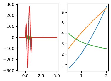
fig, axs = plt.subplots(2, 2, figsize=(10, 5))
ax = axs[0,0]
ax.plot(x/L, u1/u0, label='$u_1/u_0$')
ax.plot(x/L, u10/u0, label=r"small $\nu$ approx")
ax.plot(x/L, (u-u0)/u0/lam, label="full")
ax.set(xlabel=r"$x/L$", ylabel="$u_1/u_0$")
ax.legend()
ax = axs[0, 1]
ax.plot(x/L, F1, label='$F_1$')
ax.plot(x/L, F, label="full")
ax.legend()
ax = axs[1, 0]
ax.plot(x/L, u1/u0, 'C0-')
ax.plot(x/L, u10/u0, 'C0:')
ax.plot(x/L, (u1-u10)/nu/u0, 'C1-')
ax.plot(x/L, u11/u0, 'C1:')
ax.plot(x/L, u12/u0, 'C2:')
ylim = ax.get_ylim()
ax.plot(x/L, (u1-u10-nu*u11)/nu**2/u0, 'C2-', scaley=False)
ax.set(ylim=ylim)
ax = axs[1, 1]
ax.plot(x/L, (u-u0)/lam/u0, 'C0-')
ax.plot(x/L, u1/u0, 'C0:')
ax.plot(x/L, (u-u0-lam*u1)/lam**2/u0, 'C1-')
ax.plot(x/L, u2/u0, 'C1:')
---------------------------------------------------------------------------
ImportError                               Traceback (most recent call last)
Cell In[13], line 2
      1 from functools import partial
----> 2 from scipy.integrate import cumtrapz
      3
      4 c = u0/nu - n0*mu(n0, d=1)/m/nu/u0
      5 b = (1 + (2*n0*mu(n0, d=1) + n0**2*mu(n0, d=2))/m/u0**2)/2/nu

ImportError: cannot import name 'cumtrapz' from 'scipy.integrate' (/home/docs/checkouts/readthedocs.org/user_builds/gpe/conda/latest/lib/python3.14/site-packages/scipy/integrate/__init__.py)
The following code demonstrates that the order \(λ\) solution \(u_1(x)\) gives the correct force when integrated. (There is no need to compute \(u_2(x)\).)
def get_F1(lam=lam, nu=nu, u0=u0, n0=n0, m=m, L=L, tol=1e-7):
    a = u0 - n0*mu(n0, d=1)/m/u0
    c = a/nu
    def f(x, y):
        u1, F1 = y
        du1 = V(x)/m/nu + c*u1
        dF = -lam**2 * n0 / u0 * u1 * V(x, d=1)
        return (du1, dF)

    res1 = solve_ivp(f,
        y0=[0, 0], t_span=(0, L),
        method='BDF', atol=tol, rtol=tol)
    u1, F1 = res1.y
    return F1[-1]


lams = np.linspace(0.01, 0.3, 20)
qs = [get_F1(lam=lam, tol=lam**2 * 1e-8) /
      get_F(lam=lam, tol=lam**2 * 1e-8) for lam in lams]
plt.plot(lams, qs, '-+')
plt.plot([0], [1], 'o')
plt.gca().set(xlabel=r'$\lambda$', ylabel='$F_1/F$');
---------------------------------------------------------------------------
TypeError                                 Traceback (most recent call last)
Cell In[14], line 18
     14     return F1[-1]
     15
     16
     17 lams = np.linspace(0.01, 0.3, 20)
---> 18 qs = [get_F1(lam=lam, tol=lam**2 * 1e-8) /
     19       get_F(lam=lam, tol=lam**2 * 1e-8) for lam in lams]
     20 plt.plot(lams, qs, '-+')
     21 plt.plot([0], [1], 'o')

Cell In[14], line 3, in get_F1(lam, nu, u0, n0, m, L, tol)
      1 def get_F1(lam=lam, nu=nu, u0=u0, n0=n0, m=m, L=L, tol=1e-7):
      2     a = u0 - n0*mu(n0, d=1)/m/u0
----> 3     c = a/nu
      4     def f(x, y):
      5         u1, F1 = y
      6         du1 = V(x)/m/nu + c*u1

TypeError: unsupported operand type(s) for /: 'float' and 'function'
Thus, the complete solution to order \(λ\) is to solve the following problem:
Note that the coefficient \(c\) here is generally less than zero. We can see this by noting that the speed of sound in a material is \(c_s\) is:
Thus, for subsonic flow \(u_0<c_s\), \(c<0\). We keep this sign convention to avoid many other signs below. The homogeneous solution is \(u_1(x) = Ae^{cx}\). To find the general solution, there are several options:
One is the method of variation of parameters can be used, promoting \(A → A(x)\) to find
\[\begin{gather*} u_1(x) = A(x)e^{cx}, \qquad A'(x) e^{cx} = V(x)/{mν}, \qquad A(x) = \frac{1}{mν}\int_0^xd{y}\; e^{-cy}V(y), \\ u_1(x) = \frac{1}{mν}\int_0^xd{y}\; e^{c(x-y)}V(y),\\ F = \frac{-λ^2n_0}{mu_0}\int_{0}^{L}d{x}\;\int_0^xd{y}\; e^{c(x-y)}V(y)V'(x). \end{gather*}\]The integral is over the lower triangle \(y<x\) of the box \((x, y) ∈[0, L]×[0,L]\). To better express the dimensionality of the solution, we write the potential as \(V(x) = V_0U(x/L)\) so that the shape is described by the dimensionless function \(U(\xi)\), and we introduce the dimensionless quantity \(\kappa \propto \nu\):
\[\begin{gather*} λV(x) = λV_0U(x/L), \qquad \kappa = \frac{1}{-cL} = \frac{\nu}{-aL},\\ \begin{aligned} F &= \frac{-λ^2n_0V_0^2L}{mu_0} \underbrace{\int_{0}^{1}d{x}\;\int_0^xd{y}\; e^{(y-x)/\kappa}U(y)U'(x)}_{-\kappa^2 f(\kappa, U)},\\ &= \frac{Lu_0\kappa^2}{\nu}\frac{λ^2V_0^2n_0}{mu_0^2}f(\kappa, U). \end{aligned} \end{gather*}\]While formally correct, this solution obscures the viscosity dependence. We will see below that the normalization chosen here for \(f(\kappa, U)\) makes sense in the limit of small viscosity:
\[\begin{gather*} f(\kappa, U) = -\int_{0}^{1}d{x}\;\int_0^xd{y}\; \frac{e^{(y-x)/\kappa}}{\kappa^2}U(y)U'(x) \end{gather*}\]Another is formal manipulation. We first introduce the parameter \(a=cν\) which is independent of the viscosity, then solve algebraically treating the derivative operator as a matrix:
\[\begin{align*} νu_1'(x) &= au_1(x) + V(x)/m, \\ u_1(x) &= \frac{1}{\left(1-\frac{ν}{a}\frac{d}{d{x}}\right)}\frac{-V(x)}{am},\\ &= -\frac{V(x)}{am} - \frac{νV'(x)}{a^2m} - \frac{ν^2V''(x)}{a^3m} + O(ν^3). \end{align*}\]This is nice because it immediately allows us to expand in powers of \(ν\) by expanding \(1/(1-x) =1+x+x^2+x^3+\cdots\):
\[\begin{gather*} F = \frac{λ^2n_0 V_0^2}{mau_0} \int_{0}^{1}d{x}\;\left( U(x)U'(x) - \kappa[U'(x)]^2 + \kappa^2U''(x)U'(x) + O(ν^3) \right) \end{gather*}\]Since \(U(0)=U(1)=0\), the first term, which is a total derivative \((U^2)'/2\), vanishes. This gives:
\[\begin{align*} F &= \frac{mλ^2n_0}{au_0}\frac{V_0^2}{m^2}(-\kappa)\overbrace{ \Biggl( \int_{0}^{1}d{x}\;[U'(x)]^2 -\kappa\left.\frac{[U'(x)]^2}{2}\right|_{0}^{1} +\kappa^2\int_{0}^{1}d{x}\;U'(x)U'''(x) + O(ν^3) \Biggr)}^{f(\kappa, U)}\\ &= \frac{mλ^2n_0}{au_0}\frac{ν}{a} \frac{V_0^2}{m^2L} f(\kappa, U). \end{align*}\]This justifies the form of \(f(\kappa, U)\) chosen above. If we choose a symmetric potential so that \(|U'(0)| = |U'(1)|\), then the second term vanishes, allowing us to precisely define what a small viscosity means:
\[\begin{gather*} \frac{ν^2}{a^2} \frac{\int_{0}^{L}d{x}\;V'(x)V'''(x)} {\int_{0}^{L}d{x}\;[V'(x)]^2} = \kappa^2 \frac{\int_{0}^{1}d{x}\;U'(x)U'''(x)} {\int_{0}^{1}d{x}\;[U'(x)]^2} \ll 1. \end{gather*}\]
u10 = -V(x)/a/m
u11 = -1/a * V(x, d=1)/a/m
u12 = -1/a**2 * V(x, d=2)/a/m
u13 = -1/a**3 * V(x, d=3)/a/m

plt.plot(x/L, (u1 - u10)/nu)
plt.plot(x/L, (u1 - u10 - nu*u11)/nu**2)
plt.plot(x/L, (u1 - u10 - nu*u11 - nu**2*u12)/nu**3)

coeff = m*lam**2*n0/a/u0*nu/a
t1 = np.trapz(V(x, d=1)**2, x)/m**2
t2 = np.trapz(V(x, d=1)*V(x, d=2), x)/m**2/a
t3 = np.trapz(V(x, d=1)*V(x, d=3), x)/m**2/a**2

print(f"{t1=}, {t2=}, {t3=}")

F_ = get_F(tol=1e-13)/coeff
F1_ = get_F1(tol=1e-13)/coeff
print(F_, (F_-F1_)/lam)
print(F1_, t1)
print((F1_ - t1)/nu,
      (F1_ - t1 - nu*t2)/nu**2,
      (F1_ - t1 - nu*t2 - nu**2*t3)/nu**3,
      )
---------------------------------------------------------------------------
NameError                                 Traceback (most recent call last)
Cell In[15], line 1
----> 1 u10 = -V(x)/a/m
      2 u11 = -1/a * V(x, d=1)/a/m
      3 u12 = -1/a**2 * V(x, d=2)/a/m
      4 u13 = -1/a**3 * V(x, d=3)/a/m

NameError: name 'a' is not defined
We now replace the parameter \(a\) with the speed of sound \(c_s\). The final result, to leading order in \(λ\) is:
Here we have expressed the results in terms of the dimensionless Reynold’s number \(\mathrm{Re}\) and the ratio of the speed of sound \(c_s\) to the flow \(u_0\). Note that the force diverges as the flow speed approaches the speed of sound. The dependence on the shape appears with the dimensionless parameter \(\kappa = ν/(-aL)\):
Caution: The expansion in \(\kappa \propto \nu\) here justifies our choice for the form of \(f(\kappa, U)\) and the corresponding separation of dimensionful parameters, but it turns out that this series does not converge to the solution. We now demonstrate this. Consider for example, the dimensionless potential
This solution contains the non-analytic term \(e^{-1/\kappa}\) whose Taylor series for positive \(\kappa\) is zero. Thus, the series expansion converges to the incorrect form of:
fails to converge.
def V(x, d=0):
"""Return the external potential or derivative."""
if d == 0:
return np.where(abs(2*x/L-1) < 1,
np.sin(np.pi*(x-L)/L), 0)
elif d == 1:
return np.where(abs(2*x/L-1) < 1,
np.pi/L*np.cos(np.pi*(x-L)/L), 0)
elif d == 2:
return np.where(abs(2*x/L-1) < 1,
-np.pi**2/L**2*np.sin(np.pi*(x-L)/L), 0)
elif d == 3:
return np.where(abs(2*x/L-1) < 1,
-np.pi**3/L**3*np.cos(np.pi*(x-L)/L), 0)
def get_f(nu, u0=u0, n0=n0, V0=1, L=L, m=m, lam=lam):
cs2 = n0*mu(n0, d=1)/m
coeff = nu/u0/L / (cs2/u0**2-1)**2 * lam**2 * V0**2 *n0/m/u0**2
F1 = get_F1(nu=nu, u0=u0, n0=n0, L=L, m=m, lam=lam, tol=1e-8)
kappa = nu/u0/L/(cs2/u0**2-1)
return kappa, F1/coeff
nus = np.linspace(0.1, 10.0)
kappas, fs = np.transpose([get_f(nu=nu) for nu in nus])
xs = (np.pi*kappas)**2
plt.plot(xs, fs, '.')
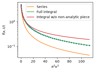
plt.plot(xs, np.pi**2/2/(1+xs), label='Series')
plt.plot(xs, np.pi**2/2
* (1 + xs - 2*kappas*(1+np.exp(-1/kappas)))
/ (1+xs)**2, label='Full integral')
plt.semilogy(xs, np.pi**2/2
* (1 + xs - 2*kappas*(1+0*np.exp(-1/kappas)))
/ (1+xs)**2, label='Integral w/o non-analytic piece')
plt.legend()
plt.gca().set(xlabel=r"$\pi^2\kappa^2$", ylabel="$f(\kappa, U)$");
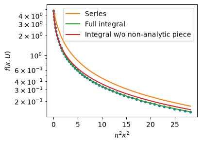
This figure shows that the integral gives the correct formula, and that for large \(\kappa\) the non-analytic piece is correct. It also shows that we have made a mistake in our series approximation. Please fix!
Here is \(U(x) = \sin^2\bigl(\pi(x-1)\bigr)\):
def V(x, d=0):
    """Return the external potential or derivative."""
    if d == 0:
        return np.where(abs(2*x/L-1) < 1,
        np.sin(np.pi*(x-L)/L)**2, 0)
    elif d == 1:
        return np.where(abs(2*x/L-1) < 1,
        np.pi/L*np.sin(2*np.pi*(x-L)/L), 0)
    elif d == 2:
        return np.where(abs(2*x/L-1) < 1,
        2*np.pi**2/L**2*np.cos(2*np.pi*(x-L)/L), 0)
    elif d == 3:
        return np.where(abs(2*x/L-1) < 1,
        -4*np.pi**3/L**3*np.sin(2*np.pi*(x-L)/L), 0)

nus = np.linspace(0.1, 10.0)
kappas, fs = np.transpose([get_f(nu=nu) for nu in nus])

xs = (2*np.pi*kappas)**2
plt.plot(xs, fs, '.')
plt.plot(xs, np.pi**2/2/(1+xs), label='Series')
plt.plot(xs, np.pi**2/2
         * (1 + xs + 2*xs*kappas*(1-np.exp(-1/kappas)))
         / (1+xs)**2, label='Full integral')
plt.semilogy(xs, np.pi**2/2
         * (1 + xs + 2*xs*kappas*(1 - 0*np.exp(-1/kappas)))
         / (1+xs)**2, label='Integral w/o non-analytic piece')
plt.legend()
plt.gca().set(xlabel=r"$\pi^2\kappa^2$", ylabel="$f(\kappa, U)$");
import sympy
x, y, k = sympy.var('x,y,kappa', positive=True)
def U(x):
    return sympy.sin(sympy.pi*(x-1))

integrand = -1/k**2 * sympy.exp((y-x)/k)*U(x).diff(x)*U(y)
f = integrand.integrate((y, 0, x)).integrate((x, 0, 1)).simplify()
display(f.factor())
display(sympy.series((1+(sympy.pi*k)**2 - 2*k)/(1+(sympy.pi*k)**2), k, 0, 10))

f_series = sum(sympy.simplify(
        (U(x).diff(*(x,)*n)*U(x).diff(x))
        .integrate((x, 0, 1))*(-k)**(n-1))
    for n in range(1, 9)[::2])
display(f_series)
If we choose \(U(\xi) = U(1-\xi)\) to be symmetric, then the even terms vanish, and we can write:
Here are a couple of special cases. Note: For numerical work, it might be better to use a potential that is sufficiently flat at the boundaries, hence the higher power. This is what I have used in the code. (Please check these.)
Thus, for a sinusoidal potential (please check):
These can also be obtained by :
import sympy
x, y, k = sympy.var('x,y,kappa', positive=True)
def U(x):
    return sympy.sin(sympy.pi*(x-1))**2

integrand = -1/k*sympy.exp((x-y)/k)*U(x).diff(x)*U(y)
display(integrand)
f = integrand.integrate((y, 0, x)).integrate((x, 0, 1))
f.expand().factor()
sympy.series(sympy.exp(1/k), k, 0, 5)
(I found these from the expansion https://oeis.org/A092812):
import numpy as np
from scipy.integrate import quad
import sympy
x, k = sympy.var('x, kappa', real=True)
V = sympy.sin(sympy.pi*(x-1))

def get_c(n):
    return k**(2*n)*(V.diff(*(x,)*(2*n+1))*V.diff(x)).integrate((x, 0, 1))

[get_c(n) for n in [0, 1, 2, 3, 4, 5]]
[pi**2/2,
 -pi**4*kappa**2/2,
 pi**6*kappa**4/2,
 -pi**8*kappa**6/2,
 pi**10*kappa**8/2,
 -pi**12*kappa**10/2]
import numpy as np
from scipy.integrate import quad
import sympy
x, k = sympy.var('x, kappa', real=True)
V = sympy.sin(sympy.pi*(x-1))**4
def get_c(n):
    f = sympy.lambdify([x], V.diff(*(x,)*(n+1))*V.diff(x))
    return int(np.round(quad(f, 0, 1)[0]) / np.pi**(n+2)) * k**(n)*sympy.pi**(n+2)
get_c(4)
4**(0-1)/2 + 2**(0-1), 5/8

sympy.simplify((1+16*x+24*x**2)/(1+4*x)/(1+16*x) - sympy.S(3)/8).factor()
from scipy.integrate import quad
def f(x):
    return V(x, d=1)**2

cs = np.sqrt(n0*mu(n0, d=1)/m)
Re = u0*L/nu
tmp = lam**2 * quad(f, 0, L)[0]
print(a/u0, (1 - (cs/u0)**2))
print(
  (1/Re) * (1/(1-(cs/u0)**2)**2) * (n0*L/m/u0**2) * tmp,
  get_F())
---------------------------------------------------------------------------
TypeError                                 Traceback (most recent call last)
Cell In[23], line 6
      2 def f(x):
      3     return V(x, d=1)**2
      4
      5 cs = np.sqrt(n0*mu(n0, d=1)/m)
----> 6 Re = u0*L/nu
      7 tmp = lam**2 * quad(f, 0, L)[0]
      8 print(a/u0, (1 - (cs/u0)**2))
      9 print(

TypeError: unsupported operand type(s) for /: 'float' and 'function'
from scipy.integrate import quad
def f(x):
    return V(x)*V(x,d=1)**2

tmp = quad(f, 0, L)[0]
lam**2*n0*nu/m/a**2/u0 * tmp, get_F()
---------------------------------------------------------------------------
TypeError                                 Traceback (most recent call last)
Cell In[24], line 5
      1 from scipy.integrate import quad
      2 def f(x):
      3     return V(x)*V(x,d=1)**2
      4
----> 5 tmp = quad(f, 0, L)[0]
      6 lam**2*n0*nu/m/a**2/u0 * tmp, get_F()

File ~/checkouts/readthedocs.org/user_builds/gpe/conda/latest/lib/python3.14/site-packages/scipy/integrate/_quadpack_py.py:479, in quad(func, a, b, args, full_output, epsabs, epsrel, limit, points, weight, wvar, wopts, maxp1, limlst, complex_func)
    476     return retval
    478 if weight is None:
--> 479     retval = _quad(func, a, b, args, full_output, epsabs, epsrel, limit,
    480                    points)
    481 else:
    482     if points is not None:

File ~/checkouts/readthedocs.org/user_builds/gpe/conda/latest/lib/python3.14/site-packages/scipy/integrate/_quadpack_py.py:626, in _quad(func, a, b, args, full_output, epsabs, epsrel, limit, points)
    624 if points is None:
    625     if infbounds == 0:
--> 626         return _quadpack._qagse(func,a,b,args,full_output,epsabs,epsrel,limit)
    627     else:
    628         return _quadpack._qagie(func, bound, infbounds, args, full_output,
    629                                 epsabs, epsrel, limit)

Cell In[24], line 3, in f(x)
      2 def f(x):
----> 3     return V(x)*V(x,d=1)**2

TypeError: 'Pow' object is not callable
A Comment on the Form of these Equations
In the applied mathematics literature, these equations are often expressed in different forms. Here we reconcile these. A standard form is:
Note that this is equivalent to our second form above after using the continuity equation:
These equations here are expressed in terms of the mass-density \(\rho = m n\) and velocity \(u\), and are usually simplified with power-law forms for \(P(\rho) = \rho^\gamma\) with \(\gamma > 1\) and \(ν(\rho) = \rho^{\alpha}\) with \(\alpha > 0\). The latter is sometimes called a Lamé viscosity.
With \(\alpha = 1\) and \(\gamma = 2\), these are equivalent to the Saint-Venant system when the pressure is quadratic \(P(\rho) = \tfrac{1}{2}\kappa \rho^2\) which is the case with the standard GPE with \(m^2 \kappa = g\):
Some references:
[Strani, 2022] uses these with the variable \(w = u\) and looks at stability properties on bounded intervals.
[Joseph et al., 2011] uses the same form \(\alpha=1\) with \(\gamma = 2/5\) to describe shockwaves in an elongated unitary Fermi gas, which has equation of state:
Note: the equation of state for the UFG is
where \([n] = 1/L^3\) is the 3D density. They argue via the Thomas-Fermi approximation that
Hence, \(\mu = \mathcal{E}'(n_{1D}) \propto n_{1D}^{2/5}\). However, see also Non-Polynomial Schrödinger Equation (NPSEQ).