Coordinate Transformations#
Here we consider solutions to time-dependent GPE-like theories of the form:
If the cloud under consideration is moving, rotating, or expanding, then one can often gain significant computational advantage by transforming the coordinates from the lab frame \(\vect{X}\) to a co-moving frame \(\vect{x}\). In some cases, it also helps to scale the wavefunction by a potentially time- and space-dependent factor \(f\):
Our goal here will be to find transformations that facilitate the numerical problem of finding \(Φ(\vect{x}, t)\).
General Transformations#
Although we will not consider changing time, we can simplify our calculations of the general transformations by adopting Einstein’s notation, letting \(X^{\mu} = (t, \vect{X})\) etc. and denoting partials \(\partial Φ/\partial t \equiv Φ_{,t}\). We then have
The transformed GPE is
If we simplify by considering only transformation of space \(x^{t}_{,t} = t_{,t} = 1\), \(x^{t}_{,i} = t_{,i} = 0\), we can re-express this as a modified GPE for \(Φ\):
The first term is a modified kinetic energy with metric \(g^{jk} = x^{j}_{,i}x^{k}_{,i}\), while the second term contains the momentum operator \(\op{p} \equiv -\I\hbar \vect{\nabla}_{x}\) multiplied by a generalized velocity \(\vect{v}\), and the last term is a corrected potential.
Alternatively, we can write \(f(X^μ) = e^{\I Θ(X^{μ})}\) (but note that \(Θ\) need not be real):
The transformed GPE is
Considering only transformation of space \(x^{t}_{,t} = t_{,t} = 1\), \(x^{t}_{,i} = t_{,i} = 0\), we have the modified GPE for \(Φ\):
Examples
Translations
Note: Although we have only derived our transformations for quadratic dispersion \(K(\op{p}) = \op{p}^2/2m\), in this case, the kinetic energy does not transform, and this remains valid for arbitrary dispersion.
Rotations Consider a rotation about a fixed axis \(\vect{\theta}\):
I.e., to work in a rotating frame, we include an angular momentum term.
Scaling
We start with a simple scaling of the coordinates – we will extend this discussion below.
More typically, as we shall see below, we include a factor \(f\) so that the density scales properly, and to remove the term linear in \(\op{p}\), but the specialization there requires assuming that the dispersion is quadratic.
Translation#
The simplest transformation corresponds to an accelerating frame:
The minimal transformation simply tracks this through the equations of motion:
The only modifications to the equation of motion are:
An addition contribution to the time dependence:
\[\begin{gather*} \I\hbar \dot{Ψ} = \I\hbar \dot{Φ} - \I\hbar \underbrace{\dot{\vect{x}}_0(t)}_{\vect{v}_0(t)} \cdot \vect{\nabla}Φ = \I\hbar \dot{Φ} + \vect{v}_0(t) \cdot \op{\vect{p}}Φ. \end{gather*}\]The potential must be evaluated in the lab-frame: \(V(\vect{X}) = V\bigl(\vect{x} - \vect{x}_0(t)\bigr)\).
Thus, in the scaled coordinates, we have
This transformation can be accounted for by simply modifying the dispersion relationship.
Where is the Acceleration?
If you are familiar with classical mechanics, you might expect a force proportional to the acceleration \(\vect{a}_0(t) = \ddot{\vect{x}}_0(t)\) contributing a linear piece to the potential \(m\vect{a}\cdot\vect{x}\). This can be recovered by including an additional phase
Including this phase gives additional pieces to the equations of motion:
Combining these we have
To recover the linear potential, we use the phase
This is more difficult to implement, but is necessary to display Galilean covariance. To see this, consider a Galilean boost \(\vect{x}_0(t) = \vect{v} t\) in a system with quadratic dispersion \(K(\op{P}) = P^2/2m\). Galilean covariance becomes manifest if we use the full transformation that includes the kinetic energy shift in the phase
Scaling (Expansion)#
If we need to scale the coordinates \(X_i = λ_i(t)x_i\) where \(\vect{X}\) is the lab frame and \(\vect{x}\) is the co-expanding frame, then we can introduce the following wavefunction:
With this transformation, the following theories are equivalent:
The utility of this transformation is that the classical behavior of an expanding gas can be modeled by setting:
which gives:
With this transformation, \(Φ(\vect{x}, t)\) evolves minimally (see [Castin and Dum, 1996]). Note that in the new coordinates, the effective trapping potential is constant, up to the overall density scaling. I.e., the time-dependence of the harmonic potential is completely absorbed into the scaling factor. This is crucial for the dr-GPE since in this co-expanding frame, the effective trap remains, even if the trap is completely turned off: \(\omega_i(t>0) = 0\).
A similar expansion can be performed scaling only \(X\) and \(Y\):
The resulting equations of motion for \(Φ(x, y, Z;t)\) can be expressed as:
This is similar to the form in [Castin and Dum, 1996], but does not include the dynamics along the \(z\) axis in the equation. A reason for using this is that the scaling transform depends on the dispersion being quadratic and we would like to explore modified dispersions (i.e. for spin-orbit coupled (SOC) BECs). In this expression, the dynamics along \(Z\) remain unscaled and explicitly managed.
A failed attempt.
One might try to express the equations simply by completely removing the potentials:
This form, however, is of little use. Consider for example an expanding cloud with \(\omega_j(t) = 0\) for \(t>0\). The resulting theory simply has no scaling, \(λ_j(t) = 1\) and degenerates to the raw GPE. We have thrown out the baby with the bath water.
Derivation#
The general derivation is a bit messy, so we start with 1D. This will also allow us to consider simultaneous scaling and translation. Let \(Ψ(X, t)\) be the physical wavefunction satisfying the non-linear Schrödinger equation, and relate this to a computational wavefunction \(Φ(x, t)\) in the computational coordinates \(x(X, t)\) with:
Expanding the Schrödinger equation
and demanding that first-order spatial derivatives \(\nabla_x Φ\) cancel (for reasons of computational efficiency), we obtain:
where primes denote derivatives with respect to \(X\).
Note
\(Θ\) is not real here – the last two terms of \(Θ\) represents an overall scaling of the wavefunction, and the integration constant \(C(t)\) is chosen here so that the evolution remains unitary. (An additional real integration constant can be introduced as a chemical potential, but it will only affect the phase of the wavefunction so we drop this.) As a consistency condition, \(\dot{C}(t)\) must not depend on \(X\), so we are restricted to coordinate transformations that have the form \(\dot{x} = [a(t)+b(t)X]x'\). This will suffice for our purposes. More general transformation will require that we allow for linear derivatives.
We now specialize to a coordinate scaling and translation:
The scaling factor \(1/\sqrt{λ}\) comes from the imaginary terms \(C(t)\) above in \(Θ\).
This leads to a effective potential of the following form:
One nice use of this is to take a problem that has a time-dependent external potential and replace it with a stationary potential. Thus, for example, suppose we have:
in the lab frame. The essence of Castin and Dumm’s argument is that a good strategy is to choose \(λ(t)\) and \(R(t)\) such that the effective potential for \(Φ\) is constant after scaling. I.e., for the GPE \(\mathcal{E}'(n) = gn\) and the equations of motion for \(Φ\) have the form:
The change in \(Φ\) is minimized if we choose
I.e., if we started in a stationary state at time \(t=0\) with external potential \(V_{\text{ext}}(0)\), then choosing such a transformation minimizes the effects of dynamics due to the trap expansion.
This gives the following differential equations for \(λ_i(t)\) and \(ρ_i(t)\):
As a simple check, consider a stationary solution in the frame where the coordinates scale to new values so that at some late time \(t\), \(λ \neq 1\) but \(\dot{λ} = \ddot{λ} = 0\). In the computational basis we should have:
Radial Expansion#
A specific use-case is that of an axially symmetric trap in which we describe the expansion in the radial direction. This is implemented in gpe/axial.py. As before, the physical coordinate \(R\) is related to the scaled coordinate \(r\) as
We discretize the equations for the scaled function \(Φ(x, r, t)\) on the scaled coordinates \(x\) and \(r\):
Note that the scaling \(λ_\perp(t)\) depends only on the trapping frequency, so can be applied to multiple components as long as the external trapping potential behaves the same way for both.
Test Examples#
In the case of expansion \(\omega_\perp(t>0) = 0\) we have:
Here we explicitly code this example so we have something to work with later.
from gpe.imports import *
from pytimeode import mixins, interfaces
from pytimeode.evolvers import EvolverABM
from mmfutils.math.bases import CylindricalBasis
@interfaces.implementer(interfaces.IStateForABMEvolvers)
class State0(mixins.ArrayStateMixin):
def __init__(self, N=2**5, R=6):
self.basis = CylindricalBasis(Nxr=(1, N),
Lxr=(1, R))
R = self.R
self.data = 5*np.exp(-R[None,:]**2/2) + 0j
@property
def R(self):
return self.basis.xyz[1].ravel()
@property
def n(self):
return abs(self[...].ravel())**2
def compute_dy_dt(self, dy):
y = self[...]
dy[...] = self.basis.laplacian(y, factor=-1./2)
dy[...] += abs(y)**2*y
dy /= 1j
return dy
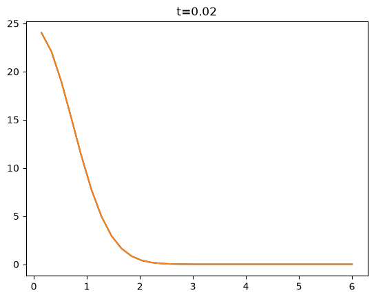
def plot(self):
plt.plot(self.R, self.n)
plt.title("t={:.4g}".format(self.t))
class State1(State0):
@property
def lam(self):
return np.sqrt(1+self.t**2)
@property
def R(self):
return self.basis.xyz[1].ravel() * self.lam
@property
def n(self):
return abs(self[...].ravel())**2 / self.lam**2
def compute_dy_dt(self, dy):
x, r = self.basis.xyz
y = self[...]
dy[...] = self.basis.laplacian(y, factor=-1./2)
dy[...] += (r**2/2.0 + abs(y)**2)*y
dy /= self.lam**2
dy /= 1j
return dy
s0 = State0()
s1 = State1()
dt = 0.0001
steps = 200
e0 = EvolverABM(s0, dt=dt)
e1 = EvolverABM(s1, dt=dt)
#fig = plt.figure(figsize=(10,5))
with NoInterrupt() as interrupted:
while not interrupted and e0.t < 1:
e0.evolve(steps)
e1.evolve(steps)
plt.clf()
e0.y.plot()
e1.y.plot()
display(plt.gcf())
clear_output(wait=True)
Here we do the same thing with the axial.State2Axial class:
from gpe.imports import *
from gpe import bec2, axial;reload(bec2); reload(axial)
from gpe.axial import u
from gpe.minimize import MinimizeState

l_unit = 1.0
t_unit = 1.0
basis = axial.CylindricalBasis(Nxr=(64, 32), Lxr=(2*6*l_unit, 6*l_unit))


class State(axial.State2Axial):
    t_expand = .0*t_unit
    _ws = np.array([48.78*0, 48.78])*u.Hz
    _ws = np.array([0.0/u.Hz, 1.0/u.Hz])*u.Hz

    def get_ws(self, t=None):
        if t is None:
            t = self.t
        if t < self.t_expand:
            return self._ws
        else:
            #return 0*self._ws
            return np.concatenate([self._ws[:1], 0*self._ws[1:]])

    def get_ws_perp(self, t=None):
        return self.get_ws(t=t)[1:]

    @property
    def ws(self):
        return self.get_ws()

    @ws.setter
    def ws(self, ws):
        pass

    def _get_Vext_(self):
        """Return (V_a, V_b, V_ab), the external potentials."""
        V_HO = (0.5*self.ms[self.bcast]
                * sum((_w*_x)**2 for _w, _x in zip(self.ws, self.xyz)))
        zero = np.zeros_like(V_HO[0])
        V_ab = self.Omega*np.exp(2j*self.k_r*self.xyz[0])
        mu_a = mu_b = 0.0
        if hasattr(self, 'mus') and self.mus:
            mu_a, mu_b = self.mus

        return (V_HO[0] - mu_a - self.delta/2.0,
                V_HO[1] - mu_b + self.delta/2.0,
                V_ab + zero)

class State_(State):
    def get_ws_perp(self, t=None):
        """Do not change these - no expansion in basis"""
        return self.get_ws(t=0)[1:]

args = dict(basis=basis, x_TF=4*u.micron, gs=[0.0007682083478971494, 0.0007682083478971494, 0])
args = dict(basis=basis, x_TF=4*u.micron, gs=[1.0, 1.0, 0.0], ms=[1.0, 1.0], Omega=0, delta=0)
s_ = State_(**args)
s = State(**args)
x, r = s.xyz
s[...] = 5/(l_unit)**1.5*np.exp(-(0*x**2+r**2)/2/l_unit**2)
s_[...] = s[...]
s.cooling_phase = s_.cooling_phase = 1.0
s.plot()
from gpe.plot_utils import MPLGrid

s0 = State0()

dt = 0.02*s.t_scale
steps = 100
e0 = EvolverABM(s0, dt=dt/t_unit)
e = EvolverABM(s, dt=dt)
e_ = EvolverABM(s_, dt=dt)

plt.figure(figsize=(15,5))
grid = MPLGrid(direction='right', space=0.2)
e.y.plot(grid=grid)
plt.plot(e0.y.R, 2*e0.y.n)
e_.y.plot(grid=grid)
plt.plot(e0.y.R, 2*e0.y.n)

with NoInterrupt() as interrupted:
    while e.y.t < 0.3*t_unit and not interrupted:
        e0.evolve(steps)
        e.evolve(steps)
        e_.evolve(steps)
        plt.figure(figsize=(15,5))
        grid = MPLGrid(direction='right', space=0.2)
        e.y.plot(grid=grid)
        plt.plot(e0.y.R, 2*e0.y.n)
        e_.y.plot(grid=grid)
        plt.plot(e0.y.R, 2*e0.y.n)
        display(plt.gcf())
        plt.close('all')
        clear_output(wait=True)
Here is a more realistic example of an expanding spherical cloud.
from gpe.imports import *
from gpe import bec2, axial;reload(bec2); reload(axial)
from gpe.axial import u
from gpe.minimize import MinimizeState

basis = axial.CylindricalBasis(Nxr=(2*64, 2*32), Lxr=(20.0*u.micron, 10*u.micron))

class State(axial.State2Axial):
    t_expand = .02*u.ms
    _ws = np.array([20*126.0, 20*126.0])*u.Hz

    def get_ws(self, t=None):
        if t is None:
            t = self.t
        if t <= self.t_expand:
            return self._ws
        else:
            return 0*self._ws
            return np.concatenate([self._ws[:1], 0*self._ws[1:]])

    def get_ws_perp(self, t=None):
        return self.get_ws(t=t)[1:]

    @property
    def ws(self):
        return self.get_ws()

    @ws.setter
    def ws(self, ws):
        pass

    def _get_Vext_(self):
        """Return (V_a, V_b, V_ab), the external potentials."""
        V_HO = (0.5*self.ms[self.bcast]
                * sum((_w*_x)**2 for _w, _x in zip(self.ws, self.xyz)))
        zero = np.zeros_like(V_HO[0])
        V_ab = self.Omega*np.exp(2j*self.k_r*self.xyz[0])
        mu_a = mu_b = 0.0
        if hasattr(self, 'mus') and self.mus:
            mu_a, mu_b = self.mus

        return (V_HO[0] - mu_a - self.delta/2.0,
                V_HO[1] - mu_b + self.delta/2.0,
                V_ab + zero)

class State_(State):
    def get_ws_perp(self, t=None):
        """Do not change these - no expansion in basis"""
        return self.get_ws(t=0)[1:]

args = dict(basis=basis, x_TF=4*u.micron)
s_ = State_(**args)
s = State(**args)
s.plot()
m = MinimizeState(s, fix_N=True)
assert m.check()
def callback(s, n=[0]):
    if n[0] % 200 == 0:
        plt.clf()
        s.plot()
        display(plt.gcf())
        plt.close('all')
        clear_output(wait=True)
    n[0] += 1
s = m.minimize(callback=callback, use_scipy=True)
s_[...] = s[...]
s.cooling_phase = s_.cooling_phase = 1.0
xi = np.sqrt(s.hbar**2/2/s.ms[0]/(s.gs[0]*s.get_density().max()))
from gpe.plot_utils import MPLGrid
dt = 0.1*s.t_scale
steps = 10
e = EvolverABM(s, dt=dt)
e_ = EvolverABM(s_, dt=dt)
with NoInterrupt() as interrupted:
    while e.y.t < 0.5*u.ms and not interrupted:
        e.evolve(steps)
        e_.evolve(steps)
        plt.figure(figsize=(15,5))
        grid = MPLGrid(direction='right', space=0.2)
        e.y.plot(grid=grid)
        e_.y.plot(grid=grid)
        display(plt.gcf())
        plt.close('all')
        clear_output(wait=True)
Expansion#
If we consider pure expansion from a static trap with \(\omega_j(t>0) = 0\) and equal radial frequencies \(\omega_x = \omega_y = \omega_\perp\), then we have the following scaling parameters in the two cases:
from scipy.integrate import odeint

from gpe import bec, minimize


class State(bec.State):
    """Here we simulate the state Phi(X, y, z) discussed above with
    explicit scaling dependence added (in y and z).

    Note: self.xyz == (X, y, z)
    """
    def init(self):
        lams = np.ones(self.dim)
        dlams = np.zeros(self.dim)
        self._lambda_cache = (0, np.ravel([lams, dlams]))
        super().init()

    def _get_Vext_(self):
        return sum(self.m*(_w*_x)**2/2.0
                   for _w, _x in zip(self.ws, self.xyz))

    def get_ws(self, t=None):
        if t is None:
            t = self.t
        if t <= 0:
            return self.ws
        else:
            return np.zeros(self.dim)

    def _rhs(self, q, t):
        """RHS for lambda(t) ODE."""
        lams, dlams =np.reshape(q, (2, self.dim))
        w0s = self.get_ws(t=0)
        ws = self.get_ws(t=t)
        ddlams = -lams * ws**2 + w0s**2/np.prod(lams)/lams
        return np.ravel([dlams, ddlams])

    def get_lambdas(self):
        if _t != self._lambda_cache[0]:
            t0, q0 = self._lambda_cache
            q1 = odeint(self._rhs, q0, [t0, self.t])[-1]
            self._lambda_cache = (t1, q1)
        return self._lambda_cache[1][:self.dim]

s = State()
s0 = minimize.MinimizeState(s).minimize()
s0.plot()
Summary#
Time-Dependent Harmonic Trap#
import sympy

sympy.init_printing()
t = sympy.var("t", real=True)
Xs = sympy.var("X, Y, Z", real=True)
xs_ = sympy.var("x, y, z", real=True)
ws = sympy.var("omega_x, omega_y, omega_z", real=True)
Ve = sympy.var("V_{ext}", cls=sympy.Function)
ls = [_l(t) for _l in sympy.var('lambda_x, lambda_y, lambda_z', cls=sympy.Function)]
xs = [_X / _l for _X, _l in zip(Xs, ls)]
m, h = sympy.var("m, hbar", positive=True)
theta = m / 2 / h * sum(_X**2 * _l.diff(t) / _l for _X, _l in zip(Xs, ls))
Phi = sympy.var("Phi", cls=sympy.Function)(*(xs + [t]))
s = sympy.sqrt(sympy.prod(ls))
Psi = sympy.exp(sympy.I * theta) * Phi / s
V = sum(m * _w**2 * _X**2 / 2 for _w, _X in zip(ws, Xs)) + Ve(*Xs)
L = (
    (
        sympy.I * h * Psi.diff(t)
        - (-(h**2) * (sum(Psi.diff(_X, _X) for _X in Xs)) / 2 / m + V * Psi)
    )
    / Psi
    * Phi
)
# display(sympy.simplify(sympy.I*h*Psi.diff(t).doit()))
subs = {_X: _x * _l for _X, _x, _l in zip(Xs, xs_, ls)}
L = L.subs(subs)
xs = xs_

# Here is the Lagrangian for Phi
Phi = Phi.subs(subs)
L0 = (
    sympy.I * h * Phi.diff(t)
    - (
        -(h**2) * (sum(Phi.diff(_x, _x) / _l**2 for _x, _l in zip(xs, ls))) / 2 / m
        + Ve(*Xs) * Phi
    )
).subs(subs)

sympy.simplify((L - L0).doit())
sympy.simplify((L).doit())
Demonstration#
from gpe import bec
from gpe.utils import GPUHelper
from gpe.contexts import FPS

reload(bec)
u = bec.u

class StateMixin(GPUHelper):
    ws = 2 * np.pi * np.array([np.sqrt(8) * 126.0, 126.0, 126.0]) * u.Hz
    def get_ws(self, t=None):
        if t is None:
            t = self.t
        if t <= 0:
            return self.ws
        else:
            return 1.5 * self.ws

    def get_Vext_GPU(self):
        ws = self.get_ws()
        xyz = self.get_xyz_GPU()
        V_trap = 0.5 * self.m * sum((_w * _x) ** 2 for _w, _x in zip(ws, xyz))

        # Arbitrary time-dependence to show that this still works.
        V_trap += 0.5 * np.sin(self.t) * np.exp(-xyz[0] ** 2 / 2)
        # V_trap += 0.5*np.exp(-self.xyz[0]**2/2)
        return V_trap


class State(StateMixin, bec.State):
    pass


class StateScale(StateMixin, bec.StateScaleHO):
    pass


args = dict(Nxyz=(32, 32, 32))
args = dict(Nxyz=(128,), x_TF=10.0)
s0 = State(**args)
s1 = StateScale(**args)


def plot(s):
    n = s.get_density()
    plt.subplot(221)
    x, y, z = list(map(np.ravel, s.xyz))
    imcontourf(y, z, n.max(axis=0), aspect=1)
    plt.subplot(222)
    imcontourf(x, z, n.max(axis=1), aspect=1)
    plt.subplot(223)
    imcontourf(x, y, n.max(axis=2), aspect=1)


dT = 0.1
dt = 0.1 * s0.t_scale
steps = int(np.ceil(dT/dt))
dt = dT/steps
e0 = EvolverABM(MinimizeState(s0).minimize(), dt=dt)
e1 = EvolverABM(MinimizeState(s1).minimize(), dt=dt)
# e0 = EvolverABM(s0, dt=0.4*s0.t_scale)
# e1 = EvolverABM(s1, dt=0.4*s1.t_scale)
clear_output()
e0.evolve(900)
e1.evolve(900)
e0.y.get_energy(), e1.y.get_energy()
T = 800
Nt = int(T/dT)
fig, ax = plt.subplots()
for frame in FPS(range(Nt), fig=fig, display=True):
    e0.evolve(steps)
    e1.evolve(steps)
    x0 = e0.y.xyz[0]
    x1 = e1.y.xyz[0]
    ax.cla()
    axs = e0.y.plot(axs=[ax])
    e1.y.plot(axs=axs)
    plt.suptitle(f"{e0.y.get_energy(), e1.y.get_energy()}")
Harmonic Traps#
Integrating the middle term by parts we get:
Let \(\vect{X} = (X, Y, Z)\) be the physical coordinates. In a time-varying harmonic potential, [Castin and Dum, 1996] provide the following alternative description in terms of scaled coordinates:
using the rescaled function \(\Phi(\vect{x}, t)\):
Let \(s = \sqrt{\lambda_x(t)\lambda_y(t)\lambda_z(t)}\), then
The energy is
Radial Expansion#
Consider the following GPE in an axially confining harmonic trap:
Now consider the following transformation:
The resulting equations of motion for \(\Phi(x, y, Z;t)\) can be expressed in one of the following two forms:
This form, however, is not of particular use. Consider for example an expanding cloud with \(\omega_j(t) = 0\) for \(t>0\). The resulting theory simply has no scaling, \(\lambda_j(t) = 1\) and degenerates to the raw GPE.
Instead, we keep the \(t=0\) potentials, applying the scaling as follows:
This is similar to the form in [Castin and Dum, 1996], but does not include the dynamics along the \(z\) axis in the equation. The reason is that the scaling transform depends on the dispersion being quadratic and we would like to explore modified dispersions. Thus, the dynamics along \(Z\) remain unscaled and explicitly managed, allowing for modified dispersion (SOC) for example.
Dynamics Traps#
As similar expansion can be performed scaling only \(X\) and \(Y\):
The resulting equations of motion for \(\Phi(x, y, Z;t)\) can be expressed in one of the following two forms:
This form, however, is not of particular use. Consider for example an expanding cloud with \(\omega_j(t) = 0\) for \(t>0\). The resulting theory simply has no scaling, \(\lambda_j(t) = 1\) and degenerates to the raw GPE.
Instead, we keep the \(t=0\) potentials, applying the scaling as follows:
This is similar to the form in [Castin and Dum, 1996], but does not include the dynamics along the \(z\) axis in the equation. The reason is that the scaling transform depends on the dispersion being quadratic and we would like to explore modified dispersions. Thus, the dynamics along \(Z\) remain unscaled and explicitly managed.
Radial Expansion#
A specific use-case is that of an axially symmetric trap in which we describe the expansion in the radial direction. This is implemented in gpe/axial.py. As before, the physical coordinate \(R\) is related to the scaled coordinate \(r\) as
We discretize the equations for the scaled function \(\Phi(x, r, t)\) on the scaled coordinates \(x\) and \(r\):
Note that the scaling \(\lambda_\perp(t)\) depends only on the trapping frequency, so can be applied to multiple components as long as the external trapping potential behaves the same way for both.
Test Example#
In the case of expansion \(\omega_\perp(t>0) = 0\) we have:
Here we explicitly code this example so we have something to work with later.
%pylab inline --no-import-all

from gpe.imports import *
from pytimeode import mixins, interfaces
from pytimeode.evolvers import EvolverABM
from mmfutils.math.bases import CylindricalBasis
from zope.interface import implementer


@implementer(interfaces.IStateForABMEvolvers)
class State0(mixins.ArrayStateMixin):
    def __init__(self, N=2**5, R=6):
        self.basis = CylindricalBasis(Nxr=(1, N), Lxr=(1, R))
        R = self.R
        self.data = 5 * np.exp(-R[None, :] ** 2 / 2) + 0j

    @property
    def R(self):
        return self.basis.xyz[1].ravel()

    @property
    def n(self):
        return abs(self[...].ravel()) ** 2

    def compute_dy_dt(self, dy):
        y = self[...]
        dy[...] = self.basis.laplacian(y, factor=-1.0 / 2)
        dy[...] += abs(y) ** 2 * y
        dy /= 1j
        return dy

    def plot(self):
        plt.plot(self.R, self.n)
        plt.title("t={:.4g}".format(self.t))


@implementer(interfaces.IStateForABMEvolvers)
class State1(State0):
    @property
    def lam(self):
        return np.sqrt(1 + self.t**2)

    @property
    def R(self):
        return self.basis.xyz[1].ravel() * self.lam

    @property
    def n(self):
        return abs(self[...].ravel()) ** 2 / self.lam**2

    def compute_dy_dt(self, dy):
        x, r = self.basis.xyz
        y = self[...]
        dy[...] = self.basis.laplacian(y, factor=-1.0 / 2)
        dy[...] += (r**2 / 2.0 + abs(y) ** 2) * y
        dy /= self.lam**2
        dy /= 1j
        return dy


s0 = State0()
s1 = State1()

dt = 0.0001
steps = 200
e0 = EvolverABM(s0, dt=dt)
e1 = EvolverABM(s1, dt=dt)
# fig = plt.figure(figsize=(10,5))
with NoInterrupt() as interrupted:
    while not interrupted and e0.t < 1:
        e0.evolve(steps)
        e1.evolve(steps)

        plt.clf()
        e0.y.plot()
        e1.y.plot()
        display(plt.gcf())
        clear_output(wait=True)
Here we do the same thing with the axial.State2Axial class:
%pylab inline --no-import-all

from gpe.imports import *
from gpe import bec2, axial

reload(bec2)
reload(axial)
from gpe.axial import u
from gpe.minimize import MinimizeState

l_unit = 1.0
t_unit = 1.0
basis = axial.CylindricalBasis(Nxr=(64, 32), Lxr=(2 * 6 * l_unit, 6 * l_unit))


class State(axial.State2Axial):
    t_expand = 0.0 * t_unit
    _ws = np.array([48.78 * 0, 48.78]) * u.Hz
    _ws = np.array([0.0 / u.Hz, 1.0 / u.Hz]) * u.Hz

    def get_ws(self, t=None):
        if t is None:
            t = self.t
        if t < self.t_expand:
            return self._ws
        else:
            # return 0*self._ws
            return np.concatenate([self._ws[:1], 0 * self._ws[1:]])

    def get_ws_perp(self, t=None):
        return self.get_ws(t=t)[1:]

    @property
    def ws(self):
        return self.get_ws()

    @ws.setter
    def ws(self, ws):
        pass

    def get_Vext(self):
        """Return (V_a, V_b, V_ab), the external potentials."""
        V_HO = (
            0.5
            * self.ms[self.bcast]
            * sum((_w * _x) ** 2 for _w, _x in zip(self.ws, self.xyz))
        )
        V_ab = self.Omega * np.exp(2j * self.k_r * self.xyz[0])
        mu_a = mu_b = 0.0
        if hasattr(self, "mus") and self.mus:
            mu_a, mu_b = self.mus

        return (
            V_HO[0] - mu_a - self.delta / 2.0,
            V_HO[1] - mu_b + self.delta / 2.0,
            V_ab,
        )


class State_(State):
    def get_ws_perp(self, t=None):
        """Do not change these - no expansion in basis"""
        return self.get_ws(t=0)[1:]


args = dict(
    basis=basis, x_TF=4 * u.micron, gs=[0.0007682083478971494, 0.0007682083478971494, 0]
)
args = dict(
    basis=basis, x_TF=4 * u.micron, gs=[1.0, 1.0, 0.0], ms=[1.0, 1.0], Omega=0, delta=0
)
s_ = State_(**args)
s = State(**args)
x, r = s.xyz
s[...] = 5 / (l_unit) ** 1.5 * np.exp(-(0 * x**2 + r**2) / 2 / l_unit**2)
s_[...] = s[...]
s.cooling_phase = s_.cooling_phase = 1.0
s.plot()
from gpe.plot_utils import MPLGrid

s0 = State0()

dt = 0.02 * s.t_scale
steps = 100
e0 = EvolverABM(s0, dt=dt / t_unit)
e = EvolverABM(s, dt=dt)
e_ = EvolverABM(s_, dt=dt)

plt.figure(figsize=(15, 5))
grid = MPLGrid(direction="right", space=0.2)
e.y.plot(grid=grid)
plt.plot(e0.y.R, 2 * e0.y.n)
e_.y.plot(grid=grid)
plt.plot(e0.y.R, 2 * e0.y.n)

with NoInterrupt() as interrupted:
    while e.y.t < 0.3 * t_unit and not interrupted:
        e0.evolve(steps)
        e.evolve(steps)
        e_.evolve(steps)
        plt.figure(figsize=(15, 5))
        grid = MPLGrid(direction="right", space=0.2)
        e.y.plot(grid=grid)
        plt.plot(e0.y.R, 2 * e0.y.n)
        e_.y.plot(grid=grid)
        plt.plot(e0.y.R, 2 * e0.y.n)
        display(plt.gcf())
        plt.close("all")
        clear_output(wait=True)
Here is a more realistic example of an expanding spherical cloud.
%pylab inline --no-import-all

from gpe.imports import *
from gpe import bec2, axial

reload(bec2)
reload(axial)
from gpe.axial import u
from gpe.minimize import MinimizeState

basis = axial.CylindricalBasis(Nxr=(2 * 64, 2 * 32), Lxr=(20.0 * u.micron, 10 * u.micron))


class State(axial.State2Axial):
    t_expand = 0.02 * u.ms
    _ws = np.array([20 * 126.0, 20 * 126.0]) * u.Hz

    def get_ws(self, t=None):
        if t is None:
            t = self.t
        if t <= self.t_expand:
            return self._ws
        else:
            return 0 * self._ws
            return np.concatenate([self._ws[:1], 0 * self._ws[1:]])

    def get_ws_perp(self, t=None):
        return self.get_ws(t=t)[1:]

    @property
    def ws(self):
        return self.get_ws()

    @ws.setter
    def ws(self, ws):
        pass

    def get_Vext(self):
        """Return (V_a, V_b, V_ab), the external potentials."""
        V_HO = (
            0.5
            * self.ms[self.bcast]
            * sum((_w * _x) ** 2 for _w, _x in zip(self.ws, self.xyz))
        )
        V_ab = self.Omega * np.exp(2j * self.k_r * self.xyz[0])
        mu_a = mu_b = 0.0
        if hasattr(self, "mus") and self.mus:
            mu_a, mu_b = self.mus

        return (
            V_HO[0] - mu_a - self.delta / 2.0,
            V_HO[1] - mu_b + self.delta / 2.0,
            V_ab,
        )


class State_(State):
    def get_ws_perp(self, t=None):
        """Do not change these - no expansion in basis"""
        return self.get_ws(t=0)[1:]


args = dict(basis=basis, x_TF=4 * u.micron)
s_ = State_(**args)
s = State(**args)
s.plot()
m = MinimizeState(s, fix_N=True)
assert m.check()


def callback(s, n=[0]):
    if n[0] % 200 == 0:
        plt.clf()
        s.plot()
        display(plt.gcf())
        plt.close("all")
        clear_output(wait=True)
    n[0] += 1


s = m.minimize(callback=callback, use_scipy=True)
s_[...] = s[...]
s.cooling_phase = s_.cooling_phase = 1.0
xi = np.sqrt(s.hbar**2 / 2 / s.ms[0] / (s.gs[0] * s.get_density().max()))
from gpe.plot_utils import MPLGrid
dt = 0.1 * s.t_scale
steps = 10
e = EvolverABM(s, dt=dt)
e_ = EvolverABM(s_, dt=dt)
with NoInterrupt() as interrupted:
    while e.y.t < 0.5 * u.ms and not interrupted:
        e.evolve(steps)
        e_.evolve(steps)
        plt.figure(figsize=(15, 5))
        grid = MPLGrid(direction="right", space=0.2)
        e.y.plot(grid=grid)
        e_.y.plot(grid=grid)
        display(plt.gcf())
        plt.close("all")
        clear_output(wait=True)
Expansion#
If we consider pure expansion from a static trap with \(\omega_j(t>0) = 0\) and equal radial frequencies \(\omega_x = \omega_y = \omega_\perp\), then we have the following scaling parameters in the two cases:
%pylab inline --no-import-all
from scipy.integrate import odeint

from gpe import bec, minimize


class State(bec.State):
    """Here we simulate the state Phi(X, y, z) discussed above with
    explicit scaling dependence added (in y and z).

    Note: self.xyz == (X, y, z)
    """

    def init(self):
        lams = np.ones(self.dim)
        dlams = np.zeros(self.dim)
        self._lambda_cache = (0, np.ravel([lams, dlams]))
        bec.State.init()

    def get_Vext(self):
        return sum(self.m * (_w * _x) ** 2 / 2.0 for _w, _x in zip(self.ws, self.xyz))

    def get_ws(self, t=None):
        if t is None:
            t = self.t
        if t <= 0:
            return self.ws
        else:
            return np.zeros(self.dim)

    def _rhs(self, q, t):
        """RHS for lambda(t) ODE."""
        lams, dlams = np.reshape(q, (2, self.dim))
        w0s = self.get_ws(t=0)
        ws = self.get_ws(t=t)
        ddlams = -lams * ws**2 + w0s**2 / np.prod(lams) / lams
        return np.ravel([dlams, ddlams])

    def get_lambdas(self):
        if _t != self._lambda_cache[0]:
            t0, q0 = self._lambda_cache
            q1 = odeint(self._rhs, q0, [t0, self.t])[-1]
            self._lambda_cache = (t1, q1)
        return self._lambda_cache[1][: self.dim]


s = State()
s0 = minimize.MinimizeState(s).minimize()
s0.plot()