Numerical Scales#
Here we continue our exploration of 1D systems a bit more in depth to build some intuition about the numerical scales in the problem required to obtain high-precision results.
The GPE in a Harmonic Trap#
We start with harmonically trapped clouds in 1D:
How big of a box do we need to accurately represent the ground state in a harmonic trap?
As discussed in Getting Started with the GPE, we have several relevant length scales in addition to the oscillator length \(a_0\): the healing length \(h\), and the interparticle spacing \(1/n_0\). This suggests 2 dimensionless parameters. However, as discussed there, the GPE does not depend on the diluteness parameter \(1/hn_0\) which must be small for the GPE to be valid. Thus, we really only have a single dimensional parameter governing the interaction strength. To access this, we can choose units such that \(m = \hbar = \omega = 1\):
If we also scale the wavefunction \(u = \psi/\sqrt{N}\) the GPE becomes
The interacting system is thus described by a single dimensionless parameter:
Do It!: Exploring Parameters
Take a moment to think about how you can systematically explore systems with different
values of the parameter \(\tilde{g}\). If you use gpe.bec.GPEStateBase, then our
code is set up so you can easily specify the following parameters:
m,hbar,g: These parameters can all be directly set.Lx: This is the box length, which can be set withLxyz = (Lx,).Nx: This is the number of points in the box, which can be set withNxyz = (Nx,).w: The trap frequency can be set when usinggpe.bec.HOMixinby settingws=(wx,).
Once these are fixed, you need to specify the initial state. This can be done by
setting either x_TF or mu. This sets the Thomas-Fermi radius where
The initial state will be initialized to a Thomas-Fermi profile with this radius. After this is done, you can minimize, or scale the state as needed.
Play with these and get three converged states with \(\tilde{g} \ll 1\), \(\tilde{g} \approx 1\), and \(\tilde{g} \gg 1\). See the code below to check your convergence.
UV and IR Convergence#
There are two types of convergence: long-distance or infrared (IR) and short-distance or ultraviolet (UV).
IR convergence means your box is big enough that the boundaries do not impact your results: e.g., if you are modeling a trapped gas, then the density should fall to zero at the edge of your simulation box, otherwise probability will flow across the boundary. If you are studying physics in a periodic box (torus), then you might have no IR errors.
UV convergence means you have enough points in your grid to resolve all features. Especially important here is the healing length which sets the scale for features like solitons and vortex cores. Note that this depends on the density, so simple estimations might be tricky.
The quick and dirty way to check this convergence is to plot the log of the density as a function of position and momentum. This should fall to a sufficiently small level at the edge of the box. Due to the duality between position and momentum, the edge of the box in momentum space tells you about UV convergence.
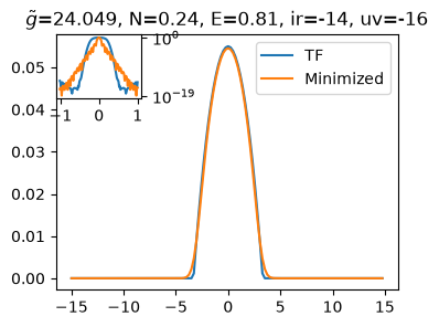
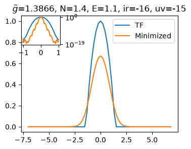
Here is a simple example:
from gpe.Examples.tutorial import StateHOConvergence1

s0 = StateHOConvergence1()
axs = s0.plot(label="TF")
s = s0.get_initialized_state()
axs = s.plot(axs=axs, label="Minimized", plot_convergence=True)
axs[0].legend();
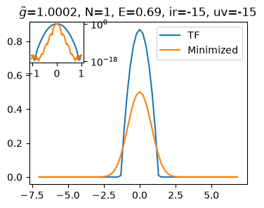
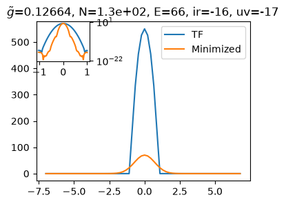
This shows a well-converged state with \(\tilde{g} \approx 1\). Try to find well-converged states with \(\tilde{g} \gg 1\) and \(\tilde{g} \ll 1\) as shown on the right by playing with the parameters. Notice how properties like the convergence, particle number, and size depend on these parameters. Note also that our initial guess is not very good if \(\tilde{g} \ll 1\).
We now try to derive some asymptotic properties to characterize the convergence starting with no interactions.
No Interactions#
In the limit of no interactions \(\tilde{g} \rightarrow 0\), then we know that the ground state is gaussian. For example, in a trap offset by \(x_0\):
To achieve relative convergence of the density \(n = \abs{\psi}^2\) to precision \(\epsilon\), we need lattice with dimensions
Lx_a0=12.01, Nx=22.95
Lx_a0=11.36, Nx=20.52
Lx_a0=10.51, Nx=17.59
Lx_a0=8.58, Nx=11.73
For \(x_0 = 0\) and precision \(\epsilon\) here are some values:
For FFT performance, we choose the smallest 5-smooth numbers: i.e. \(N_x=45\) for machine precision.
smooth_numbers=[2, 3, 4, 5, 6, 8, 9, 10, 12, 15, 16, 18, 20, 24, 25, 27, 30, 32, 36, 40, 45, 48, 50, 54, 60, 64, 72, 75, 80, 81, 90, 96]
Some Numerical Details
If we want the wavefunction to machine precision, then we need \(L_x/a_0 > 17.0\) and \(N_x > 46\), but we cannot achieve this with minimization etc. Round-off error etc. truncation at a relative precision of \(10^{-19}\) in \(n\), or \(10^{-9.5}\) in \(\psi\). For the gaussian, this corresponds to \(L_x/a_0 > 13.3\).
Well into the Thomas-Fermi regime, the chemical potential is well approximated by
with no correction \(\hbar \omega /2\). It turns out to be a safe approximation to take the box size to be \(L_x > 2R + 13.3 a_0\), but this is somewhat overkill, as we shall see.
As for UV convergence, we need
In the non-interacting limit, this gives
which is not sufficient.
Weak Interactions#
For weak interactions, we can estimate the chemical potential variationally using the gaussian ground state:
Strong Interactions#
In the limit of large \(\tilde{g}\), the states should be well approximated by the Thomas-Fermi approximation:
This gives the approximation
Full Solution#
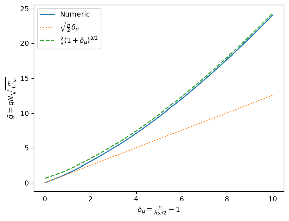
To specify the solution, it is convenient to use the dimensionless parameter \(\delta_{\mu}\):
The interaction strengths increase monotonically with \(\delta_\mu\) from the non-interacting case \(\delta_\mu = 0\). Here we plot the function \(\tilde{g}(\delta_\mu)\), which has the asymptotic forms:
import numpy as np, matplotlib.pyplot as plt
dmus = np.linspace(0.01, 10)
ss = [StateHOConvergence1(dmu=dmu).get_initialized_state() for dmu in dmus]
gs = [s.get_gtilde() for s in ss]
gs1 = np.array([np.sqrt(np.pi/2)*dmu for (s, dmu) in zip(ss, dmus)])
gs2 = 2/3*(1+dmus)**(3/2)
fig, ax = plt.subplots()
ax.plot(dmus, gs, label="Numeric")
ax.plot(dmus, gs1, ':', label=r"$\sqrt{\frac{\pi}{2}}\delta_{\mu}$")
ax.plot(dmus, gs2, '--', label=r"$\frac{2}{3}(1+\delta_{\mu})^{3/2}$")
ax.set(xlabel=r"$\delta_{\mu} = \frac{\mu}{\hbar \omega / 2} - 1$",
       ylabel=r"$\tilde{g}=gN\sqrt{\frac{m}{\hbar^3 \omega}}$")
ax.legend();
Lx = 14
dmu, dx
0.001, 29,
0.01, 31
0.1, 34
1.0, 39
10.0, 62, 20
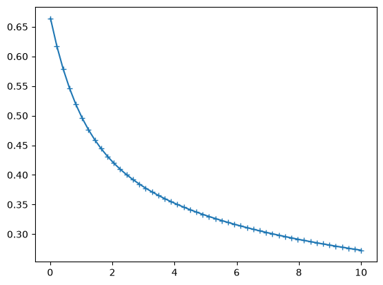
Here are the residuals: fitting these could give a nice interpolation:
plt.plot(dmus, gs2-gs, '-+')
[<matplotlib.lines.Line2D at 0x7f901a89d7f0>]
Details
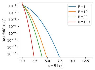
From a numerical standpoint, we would like to characterize how far beyond \(R\) we must extend the box to ensure appropriate convergence. Asymptotically, the density drops, and we can return to the gaussian approximation.
The solutions here are simply those of the harmonic oscillator \(u(x) = H_{n}(x)e^{-x^2/2}\) where \(n = \tfrac{1}{2}(R^2-1)\). Note that we thus expect fluctuations with an energy scale
The Plancherel–Rotach asymptotics for these can be derived using the WKB approximation:
This form is valid for \(x \gg R\). From the figure on the right, we confirm that \(L_x > 2R + 13.3a_0\) is safe as mentioned above, but that for larger values of \(R\), one can be more restrictive: e.g., for \(R=100\), we can take \(L_x > 2(R+2.5a_0)\).
To derive an approximation for these numerical results, we need the form for \(x \approx R\):
Thus
If \(R\gg 7.5 a_0\), then the density will fall to machine precision when \(x = R+\delta\) and \(x/R \approx 1\) so \(\varphi \approx \sqrt{2\delta / R} \ll 1\) will be small:
If we ignore the prefactor, then for machine precision, we find
which, for machine precision \(\epsilon \sim 10^{-16}\) gives \(R \delta^3 \approx 1300\), making the prefactor \(\approx 0.286 \approx 1/3\). This gives the refined approximation
Due to the approximations made by assuming large \(R\), this somewhat over-estimates the required extension for small values. Also, as discussed above, an accuracy of \(10^{-9.5}\) for \(u(x)\) is usually sufficient, which changes the factor \(11\) above to \(7.6\). Thus, we arrive at the following heuristic for the minimal box size required for the ground state:
Important
For an accurate representation of the ground state of a harmonically trapped cloud with Thomas-Fermi radius \(R\), we should use a box of length at least:
where \(a_0\) is the oscillator length.
import numpy as np
import matplotlib.pyplot as plt
from gpe.bec import StateGPEBase, HOMixin, u
from gpe.utils import get_good_N
from gpe.minimize import MinimizeState
class State(HOMixin, StateGPEBase):
"""To set the interaction strength, set `x_TF`.
We use the TF formula to get the particle number
"""
a0_micron = 1.0 # Trap length in microns.
# Here we express Lx = 2 x_TF + Lx_a0*a_0 where R is the TF radius.
Lx_a0 = 17.0 # Box length beyond R_TF
Nx = 48
N = 1.0
x_TF_micron = 4.0
n0a0 = 1.0 # Central density in units of a0
def __init__(self, **kw):
for key in list(kw):
if hasattr(self, key):
setattr(self, key, kw.pop(key))
m = u.m_Rb87
hbar = u.hbar
a0 = self.a0_micron * u.micron
w = hbar / m / a0**2
# Required by HOMixin
self.ws = (w,)
# self.healing_length = self.healing_length_micron * u.micron
# dx = self.dx_healing_length * self.healing_length
# Select a good Nx that will perform well - small prime factors.
# Nx = get_good_N(Lx / dx)
# Calculate the chemical potential and g
R = x_TF = self.x_TF_micron * u.micron
g_ = 2/3 * (R/a0)**3
N = max(1, self.n0a0 * (32 * g_ / 9) ** (1 / 3))
g = hbar**2 * g_ / N / m / a0
delta = a0 * 6.7 * min(1, 7.7/6.7 / max((R/a0)**(1/3), 1))
Lx = 2 * (x_TF + delta)
dx = Lx / self.Nx
kw.update(hbar=hbar, m=m, Lxyz=(Lx,), Nxyz=(self.Nx,), Ntot=N, g=g)
super().__init__(**kw)
def set_initial_state(self):
a0 = self.a0_micron * u.micron
x = self.get_xyz()[0]
psi = np.exp(-(x/a0)**2/2)
self.set_psi(psi)
self *= np.sqrt(self.Ntot / self.get_N())
self._N = self.get_N_GPU()
def init(self):
"""Perform any initializations before the simulation begins."""
super().init()
axs = None
#for h in [1000.0, 10.0, 1.0, 0.1, 0.01]:
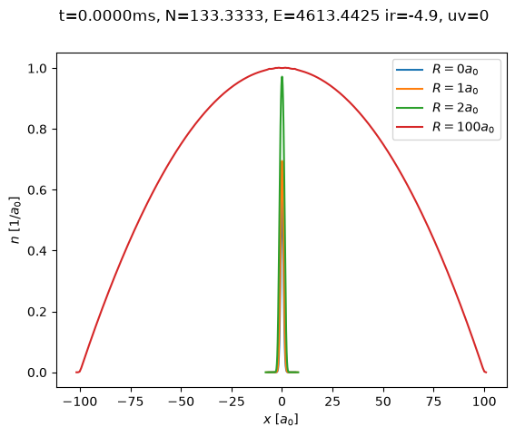
for x_TF_micron in [0, 1, 2, 100]:
s0 = State(x_TF_micron=x_TF_micron, Nx=256)
m = MinimizeState(s0, fix_N=True)
s = m.minimize()
axs = s.plot(axs=axs, label=f"$R={x_TF_micron:}a_0$")
ax = axs[0]
ax.set(xlabel="$x$ [$a_0$]", ylabel="$n$ [$1/a_0$]")
ax.legend();
plt.clf()
s0 = State(x_TF_micron=40, Nx=256*2*2)
#axs = s0.plot()
s = MinimizeState(s0, fix_N=True).minimize()
s.plot(log=True)
[<Axes: >]
a0, R = 1.0, 10.0
m, w = s.m, s.ws[0]
N = s.get_N()
g_N = s.g/N
n = np.maximum(0, s.m * s.ws[0] **2 * (R**2 - s.x**2)/2 / s.g)
np.trapezoid(n, s.x)
#plt.plot(s.x, np.maximum(0, s.m * s.ws[0] **2 * (R**2 - s.x**2)/2 / s.g))
np.float64(0.833331674859598)
2*m*w**2*R**3/3/s.g
0.8333333333333331
3/2*g_N*a0**3/R**3
np.float64(0.000258890927146747)
UV and IR Convergence#
There are two types of convergence: long-distance or infrared (IR) and short-distance or ultraviolet (UV).
IR convergence means your box is big enough that the boundaries do not impact your results: e.g., if you are modeling a trapped gas, then the density should fall to zero at the edge of your simulation box, otherwise probability will flow across the boundary. If you are studying physics in a periodic box (torus), then you might have no IR errors.
UV convergence means you have enough points in your grid to resolve all features. Especially important here is the healing length which sets the scale for features like solitons and vortex cores. Note that this depends on the density, so simple estimations might be tricky.
The quick and dirty way to check this convergence is to plot the log of the density as a function of position and momentum. This should fall to a sufficiently small level at the edge of the box. Due to the duality between position and momentum, the edge of the box in momentum space tells you about UV convergence.
Here is a simple example:
import numpy as np
import matplotlib.pyplot as plt

from pytimeode.evolvers import EvolverABM

from gpe.bec import StateGPEBase, HOMixin, u
from gpe.utils import get_good_N
from gpe.contexts import FPS

class State(HOMixin, StateGPEBase):
    Nxyz = (64*3,)
    Lxyz = (10.0*2,)
    x0_ = 0.2  # Location of soliton

    def __init__(self, **kw):
        for key in list(kw):
            if hasattr(self, key):
                setattr(self, key, kw.pop(key))

        kw.update(Nxyz=self.Nxyz, x_TF=8.0, ws=[0.5,])
        super().__init__(**kw)

    def set_initial_state(self):
        super().set_initial_state()
        x = self.get_xyz()[0]
        x0 = self.x0_ * x.max()
        psi = self.get_psi()
        self.set_psi(psi * np.where(x<x0, -1, 1))
        self._N = self.get_N_GPU()

    def plot_convergence(self, axs=None, **kw):
        if ax is None:
            fig, ax = plt.subplots()
        x = self.get_xyz()[0].ravel()
        k = np.fft.fftshift(self.basis.kx.ravel())
        n_x = abs(self.get_psi())**2
        n_k = np.fft.fftshift(abs(self.basis.fftn(self.get_psi()))**2)
        ax.semilogy(x/abs(x.max()), n_x/n_x.max(), label='IR', **kw)
        ax.semilogy(k/abs(k.max()), n_k/n_k.max(), label='UV', **kw)
        ax.legend()
        return ax

    def plot(self, ax=None, **kw):
        if ax is None:
            fig, ax = plt.subplots()
        x = self.get_xyz()[0].ravel()
        n = self.get_density()
        ax.plot(x, n, **kw)
        N, E, t = self.get_N(), self.get_energy(), self.t
        ax.set(title=f"{t=:.4f}, {N=:.4f}, {E=:.4f}")
        return ax


s0 = State()
s0.cooling_phase = 1j
s0.init()

ev = EvolverABM(s0, dt=0.5*s0.t_scale)
fig, ax = plt.subplots(figsize=(4,3))
ev.y.plot_convergence(ax=ax)
for n in FPS(range(31), fig=fig, embed=True, display=True):
    ev.evolve(40)
    ax.cla()
    ev.y.plot_convergence(ax=ax)
    E = ev.y.get_energy()
    ax.set(title=f"Step {2*n}, {E=:.4f}", ylim=(1e-16, 1))

s = State()
s.set_psi(ev.y.get_psi());
---------------------------------------------------------------------------
UnboundLocalError                         Traceback (most recent call last)
Cell In[16], line 60
     56 s0.init()
     57
     58 ev = EvolverABM(s0, dt=0.5*s0.t_scale)
     59 fig, ax = plt.subplots(figsize=(4,3))
---> 60 ev.y.plot_convergence(ax=ax)
     61 for n in FPS(range(31), fig=fig, embed=True, display=True):
     62     ev.evolve(40)
     63     ax.cla()

Cell In[16], line 32, in State.plot_convergence(self, axs, **kw)
     31     def plot_convergence(self, axs=None, **kw):
---> 32         if ax is None:
     33             fig, ax = plt.subplots()
     34         x = self.get_xyz()[0].ravel()
     35         k = np.fft.fftshift(self.basis.kx.ravel())

UnboundLocalError: cannot access local variable 'ax' where it is not associated with a value
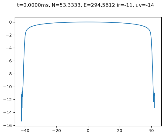
Here we imprint a soliton on a TF background: this initial state has kinks, leading to poor UV convergence. We then apply 60 steps with imaginary time evolution, which cools the state, allowing us to achieve both UV and IR convergence.
fig, ax = plt.subplots(figsize=(4,3))
s0.plot_convergence(ax=ax)
s.plot_convergence(ax=ax, ls='--');
---------------------------------------------------------------------------
UnboundLocalError                         Traceback (most recent call last)
Cell In[17], line 2
      1 fig, ax = plt.subplots(figsize=(4,3))
----> 2 s0.plot_convergence(ax=ax)
      3 s.plot_convergence(ax=ax, ls='--');

Cell In[16], line 32, in State.plot_convergence(self, axs, **kw)
     31     def plot_convergence(self, axs=None, **kw):
---> 32         if ax is None:
     33             fig, ax = plt.subplots()
     34         x = self.get_xyz()[0].ravel()
     35         k = np.fft.fftshift(self.basis.kx.ravel())

UnboundLocalError: cannot access local variable 'ax' where it is not associated with a value
In the margin, we compares the convergence of the initial state (solid) to the state after cooling (dashed). Note that, although the initial state has compact support, and is thus IR converged, the presence of high frequency modes immediately spoils this during as seen above.
Now we can look at the dynamics of this state:
T = 2*np.pi / s.ws[0]
dT = T/10
dt = 0.4*s.t_scale
steps = int(np.ceil(dT/dt))
dt = dT/steps
ev = EvolverABM(s, dt=dt)
fig, ax = plt.subplots(figsize=(4,3))
for n in FPS(range(10*4), fig=fig, embed=True, display=True):
    ev.evolve(steps)
    ax.cla()
    ev.y.plot(ax=ax)
/home/docs/checkouts/readthedocs.org/user_builds/gpe/conda/latest/lib/python3.14/site-packages/gpe/bec.py:246: RuntimeWarning: overflow encountered in multiply
  self.data *= V
WARNING:matplotlib.animation:MovieWriter stderr:
[in#0 @ 0x5b9003b96e80] Could find no file or sequence with path '/tmp/tmpnb3u_wax/tmp%07d.png' and index in the range 0-4
[in#0 @ 0x5b9003b96b40] Error opening input: No such file or directory
Error opening input file /tmp/tmpnb3u_wax/tmp%07d.png.
Error opening input files: No such file or directory
Exception ignored while closing generator <generator object FPS.__iter__ at 0x7f9019a16020>:
Traceback (most recent call last):
  File "/home/docs/checkouts/readthedocs.org/user_builds/gpe/conda/latest/lib/python3.14/site-packages/mmf_contexts/contexts.py", line 1221, in __iter__
    with self._writer(outfile=outfile):
  File "/home/docs/checkouts/readthedocs.org/user_builds/gpe/conda/latest/lib/python3.14/contextlib.py", line 162, in __exit__
    self.gen.throw(value)
  File "/home/docs/checkouts/readthedocs.org/user_builds/gpe/conda/latest/lib/python3.14/site-packages/matplotlib/animation.py", line 228, in saving
    self.finish()
  File "/home/docs/checkouts/readthedocs.org/user_builds/gpe/conda/latest/lib/python3.14/site-packages/matplotlib/animation.py", line 472, in finish
    super().finish()
  File "/home/docs/checkouts/readthedocs.org/user_builds/gpe/conda/latest/lib/python3.14/site-packages/matplotlib/animation.py", line 343, in finish
    raise subprocess.CalledProcessError(
subprocess.CalledProcessError: Command '['ffmpeg', '-framerate', '10', '-i', '/tmp/tmpnb3u_wax/tmp%07d.png', '-loglevel', 'error', '-vcodec', 'h264', '-pix_fmt', 'yuv420p', '-metadata', 'title=Movie generated with the animate library.', '-metadata', 'artist=Unknown.', '-metadata', 'comment=', '-y', PosixPath('/tmp/tmph4dsts1h/temp_FPS_movie.m4v')]' returned non-zero exit status 254.
---------------------------------------------------------------------------
AssertionError                            Traceback (most recent call last)
Cell In[18], line 9
      5 dt = dT/steps
      6 ev = EvolverABM(s, dt=dt)
      7 fig, ax = plt.subplots(figsize=(4,3))
      8 for n in FPS(range(10*4), fig=fig, embed=True, display=True):
----> 9     ev.evolve(steps)
     10     ax.cla()
     11     ev.y.plot(ax=ax)

File ~/checkouts/readthedocs.org/user_builds/gpe/conda/latest/lib/python3.14/site-packages/pytimeode/evolvers.py:411, in EvolverABM.evolve(self, steps)
    409 getattr(self.y, "pre_evolve_hook", lambda: None)()
    410 for kt in range(steps):
--> 411     self.do_step()
    412 assert np.allclose(self.y.t, t0 + steps * self.dt)
    414 getattr(self.y, "post_evolve_hook", lambda: None)()

File ~/checkouts/readthedocs.org/user_builds/gpe/conda/latest/lib/python3.14/site-packages/pytimeode/evolvers.py:427, in EvolverABM.do_step(self)
    424         self.dcps = [0 * _y for _y in self.ys]
    425 else:
    426     # self.do_step_ABM()
--> 427     self.do_step_ABM_apply()

File ~/checkouts/readthedocs.org/user_builds/gpe/conda/latest/lib/python3.14/site-packages/pytimeode/evolvers.py:594, in EvolverABM.do_step_ABM_apply(self)
    591 y.t = t + dt
    593 dy = dys.pop()
--> 594 dy = self.get_dy(y=y, dy=dy)
    596 ys.insert(0, y)
    597 dys.insert(0, dy)

File ~/checkouts/readthedocs.org/user_builds/gpe/conda/latest/lib/python3.14/site-packages/pytimeode/evolvers.py:106, in EvolverBase.get_dy(self, y, t, dy)
    103     dy.t = y.t
    105 with y.lock:
--> 106     dy = y.compute_dy_dt(dy=dy)
    107     if dy is None:
    108         raise ValueError("compute_dy_dt must return a state (got None)")

File ~/checkouts/readthedocs.org/user_builds/gpe/conda/latest/lib/python3.14/site-packages/gpe/bec.py:804, in _StateBase.compute_dy_dt(self, dy, subtract_mu)
    802         mu = mu.real
    803     else:
--> 804         assert np.allclose(0, mu.imag / (abs(mu) + 1))
    805 elif not self.constraint:
    806     mu = 0

AssertionError: