Viscosity Notes 4#
These are some supporting notes for the document Effective Viscosity.
Saint-Venant Equations: Vacuum Interface#
In Viscosity Notes 3 we explored the Saint-Venant equations in the case where the density \(n > 0\) was finite everywhere. The case where \(n = 0\) – sometimes referred to as “dry bed” problems – can pose a challenge. To see if we have an issue here, we simulate the dam breaking problem:
Wet bed: nR=0.1: nfev = 3188
Dry bed: nR=0.001: nfev = 4169
CPU times: user 38.8 s, sys: 743 ms, total: 39.6 s
Wall time: 23.3 s
Notice that the initial step for the dry bed \(n_R=0.001\) takes an order of magnitude more
function evaluations (nfev) than the wet bed \(n_R=0.1\). As we make the bed dryer,
this gets even worse. One approach to dealing with this is to reformulate the problem
with Lagrangian fluid dynamics.
Lagrangian Fluid Dynamics#
There are two alternative formulations of fluid dynamics. The Eulerian approach we have adopted so far describes the density and velocity as functions of fixed spatial position. The Lagrangian approach instead follows the particle motion. Thus, consider the position \(x = X(x_0, t)\) of the fluid element that started at \(x_0\) at time \(t=0\): \(X(x_0, 0) = x_0\). The relationship between the two is expressed in terms of the velocity
Intuition
The Lagrangian description is actually the more physically natural one. Taken to its extreme, it simply describes the motion of the fluid particles using Newton’s law: \(F = ma = m X_{,tt}\). One has particle conservation “for free” since the number of particles is explicitly conserved – they just move around.
What is tricky is computing the force. At a microscopic level, this is just the inter-particle interactions: I.e., the van der Waals force between the fluid particles. Of course, we do not have the resources to describe the moles of particles in a typical fluid, so we must instead break the fluid up into small chunks – fluid elements – that we assume stay together during the course of the evolution. The net force on such an element is obtained by averaging over the microscopic forces, and is expressed instead in terms of the equation of state and gradient of the external potential. For a recent attempt to derive these forces from an averaging procedure, see [Deng et al., 2025].
In our Lagrangian approach, we characterize the locations \(X(x_0, t)\) of the center-of-mass of the fluid element that started at position \(x_0\), and track its motion over time, assuming that it “stays together”, thus, the original density \(n_0(x_0)\) is stretched by the factor \(X_{,x_0}\). This is very much in the spirit of smoothed-particle hydrodynamics (SPH).
A more flexible – but complicated – approach would be to track the boundaries of each fluid element, allowing fluid to flow from one to the other. This approach would allow us to relax the mesh as a simulation evolved, but we will not discuss it here.
The following differential is useful:
This gives us the following differentiation rules
(In the second form, we suppress arguments – everything on the right-hand side in the Lagrangian framework is a function of \(x_0\) and \(t\), while everything on the left-hand side is formulated in the Eulerian framework as a function of \(x\) and \(t\).)
Thus, we can convert from Eulerian to Lagrangian with the following formulae:
As a check, note the physical content of the last two equations. The second is just the continuity equation \(n_{,t} = -(nu)_{,x}\), while the first shows that the covariant (material) derivative is just the acceleration of the fluid elements:
For the viscosity term, we need one more:
Thus, the hydrodynamic formulation is
While one could write this out explicitly, we keep this form and compute the various parts independently.
Vacuum Interface#
The advantage of the Lagrangian formulation is that we can now model the vacuum interface. A simple example is if we have a fluid that is initially confined to some compact region, then the boundary will follow the evolution of the outermost fluid elements. For this to work, we must be careful about the boundary conditions.
Todo
Ed: Explore and make rigorous the boundary conditions.
Numerical Implementation#
Here we demonstrate an initial numerical simulation using a finite-difference approach. We model a harmonically trapped gas with a small bump in the middle, starting from the ground state but suddenly moving the potential. Without the bump, the solution will smoothly oscillate back and forth with a constant velocity profile, hence without any dissipation since our viscosity term contains \(u_{,x} = 0\): the bump will break this uniformity, inducing drag, and slowing the motion.
Nx = 128
x0 = np.linspace(-1.0, 1.0, Nx)
dx0 = np.diff(x0).mean()

g_m = 1.0  # Coupling constant g/m
nu = 0.2  # Viscosity coefficient

w = np.sqrt(2)  # Trap frequency
V0_m = 0.5  # Bump height
sigma = 0.1  # Bump width

# Initial density provile
X0_shift = 0.5  # Initial shift of the cloud
X0 = x0 + X0_shift
n0 = w**2/2/g_m * (1 - x0**2)
n0_x0 = -w**2 / g_m * x0

# Finite difference approximations for the derivatives
o = np.ones(Nx)
Df = (np.diag(o[1:], 1) - np.diag(o, 0))/dx0
Db = (np.diag(o, 0) - np.diag(o[:-1], -1))/dx0
Dc = (Df + Db)/2
D2 = Db @ Df

# Free bc's (second derivative is zero).
Dc[0, :2] = [-1/dx0, 1/dx0]
Dc[-1, -2:] = [-1/dx0, 1/dx0]
D2[0, :] = 0
D2[-1, :] = 0

def pack(X, X_t):
    return np.ravel([X, X_t])

def unpack(y):
    return np.reshape(y, (2, Nx))

def unpack_xnu(y):
    X, X_t = unpack(y)
    X_x0 = Dc @ X
    n = n0 / X_x0
    u = X_t
    x = X
    return x, n, u

def compute_dy_dt(t, y):
    X, X_t = unpack(y)
    X_x0 = Dc @ X
    X_x0x0 = D2 @ X
    n_x = n0_x0 / X_x0**2 - n0 * X_x0x0 / X_x0**3

    u_xx = (D2 @ X_t) / X_x0**2 - Dc @ X_t * X_x0x0 / X_x0**3
    a_ext = - w**2 * X
    a_ext += V0_m * np.exp(-X**2/2/sigma**2) * X/sigma**2
    X_tt = a_ext - g_m * n_x + nu * u_xx
    return pack(X_t, X_tt)
res.nfev=1177
res.nfev=3418
CPU times: user 10.3 s, sys: 6.41 ms, total: 10.3 s
Wall time: 5.2 s
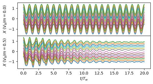
Now we show the animation:
CPU times: user 23 s, sys: 501 ms, total: 23.6 s
Wall time: 23.8 s
Spectral Basis#
The finite difference approach used above works reasonably well, but we would like to see if we could apply a spectral method using a Spectral Methods: Chebyshev Basis. We do this here, imposing zero Laplacian boundary conditions
import scipy.fft
sp = scipy

Nx = 128
th0 = (2*np.arange(Nx) + 1) * np.pi / 2 / Nx
k = np.arange(Nx)
x0 = np.cos(th0)

X0_shift = 0.5  # Initial shift of the cloud
X0 = x0 + X0_shift

# Initial density provile
n0 = w**2/2/g_m * (1 - x0**2)
n0_x0 = -w**2 / g_m * x0

# To do: Make this work with arrays f.
def diff(f, d=1, k=k, th=th0):
    ft = sp.fft.dct(f, type=2, norm='forward')
    s = np.sin(th)

    # Shift the coefficients and pad with zero.
    df_dth = sp.fft.dst(np.concatenate([-(ft*k)[1:], [0]]), type=3)
    if d == 1:
        df_dx = -df_dth / s
        return df_dx
    elif d == 2:
        d2f_dth2 = sp.fft.idct(-ft*k**2, type=2, norm='forward')
        d2f_dx2 = (d2f_dth2 - df_dth / np.tan(th)) / s**2
        return d2f_dx2
    return diff(df_dx, d=d-1)

def unpack_xnu(y):
    X, X_t = unpack(y)
    X_x0 = np.array([diff(x) for x in X])
    n = n0 / X_x0
    u = X_t
    x = X
    return x, n, u

def compute_dy_dt(t, y):
    X, X_t = unpack(y)
    X_x0 = diff(X)
    X_x0x0 = diff(X, d=2)
    n_x = n0_x0 / X_x0**2 - n0 * X_x0x0 / X_x0**3

    u_xx = (diff(X_t, d=2)) / X_x0**2 - diff(X_t) * X_x0x0 / X_x0**3
    # Zero-laplacian boundary conditions
    u_xx[0] = u_xx[-1] = 0

    a_ext = - w**2 * X
    a_ext += V0_m * np.exp(-X**2/2/sigma**2) * X/sigma**2
    X_tt = a_ext - g_m * n_x + nu * u_xx
    return pack(X_t, X_tt)
res.nfev=1206
res.nfev=4458
CPU times: user 47.6 s, sys: 38 ms, total: 47.7 s
Wall time: 24 s
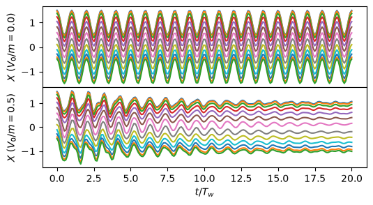
Now we show the animation:
:tags: [hide-input]
# We don't actually execute this to save time... it looks the same as the previous movie.
%%time
data = []
for i, (V0_m, res) in enumerate(ress):
    X, X_t = res.y.reshape((2, Nx, Nt))
    X_x0 = np.transpose([diff(x) for x in X.T])
    n = n0[:, None] / X_x0

    x_ = np.linspace(X.min(), X.max(), 200)
    V_ext = w**2 * X**2 / 2
    V_ext += V0_m * np.exp(-X**2/2/sigma**2)
    b = V_ext / g_m

    b_ = w**2 * x_**2 / 2
    b_ += V0_m * np.exp(-x_**2/2/sigma**2)
    b_ /= g_m

    h = b + n

    data.append((V0_m, x_, b_, X, b, h))

fig, axs = plt.subplots(1, 2, figsize=(6, 3), sharey=True, constrained_layout=True)
for i in FPS(Nt, fig=fig, embed=True, fps=10):
    t = ts[i]
    for ax, (V0_m, x_, b_, X, b, h) in zip(axs, data):
        ax.cla()
        ax.plot(x_, b_, 'k-')
        ax.fill_between(X[:, i], b[:, i], h[:, i], color='cyan')
        ax.set(title=f"$V_0/m = {V0_m:.1f}$", xlabel="$x$",
               xlim=(X.min(), X.max()), ylim=(0, h.max()))
    fig.suptitle(rf"$t={t/Tw:.2f}T_{{\omega}}$")
Comparison#
Let’s now do a comparison between the codes using the code in viscosity.py. We start
with flow over a barrier in a periodic box.
import viscosity
class Flow(viscosity.FlowBase):
    Nx = 128
    xR = 5.0
    xL = -5.0
    Basis = viscosity.BasisFFT

    n0 = 1.0
    v0 = 0.0

    # Potential
    V0 = 0.1
    V_sigma = 1.0
    V_grad = 0.2

    def init(self):
        self.basis = self.Basis(Nx=self.Nx, Lx=self.xR - self.xL, xL=self.xL)
        x = self.basis.x
        zero = np.zeros_like(x)
        self.y0 = self.pack(self.n0 + zero, self.v0 + zero)

    def get_Vext(self, x, t, d=0):
        if d == 0:
            return self.V0 * np.exp(-(x/self.V_sigma)**2/2) + x*self.V_grad
        elif d == 1:
            return - self.V0 * x / self.V_sigma**2 * np.exp(-(x/self.V_sigma)**2/2) + x
        else:
            raise NotImemplementedError
f = Flow()
Restructuring the Grid#
The Lagragian approach seems to work quite well, but the resulting meshes can end up being quite distorted – especially if shockwaves present – leading to numerical instabilities. The problem is that the Lagrangian framework naturally puts particles where the density is high, but we need instead lots of grid points where the gradient or curvature of the density is high.
Consider the state at time \(t\) (which we will suppress now). The Lagrangian approach encodes the density in the functions \(X(x_0)\) and \(\dot{X}(x_0)\) of the initial coordinate \(x_0\), along with the initial density profile \(n_0(x_0)\):
The same state can be described by a new pair of functions \(Y(y_0)\) and \(\tilde{n}_0(y_0)\) if
where
Systematic Solution
It can be productive to develop intuitions where you can solve these problems quickly with shortcuts. This allows you to quickly explore different options and discard false starts. But when you are stuck, having a systematic approach is also useful.
To proceed systematically, we note that \(x_0\) is a dummy variable, thus the total variation of the physical density \(\d{n} = 0\) should be zero:
This requires that
One can proceed systematically to solve this, but some insight might be gained by considering a similar type of equation:
This is thus solved by constant \(fg\). Here we have the wrong sign, but recall that signs come from the exponents: \((fg^a)' = f'g^a + afg^{a-1}g'\). Dividing by the ugly factor of \(g^{a-1}\), we have
Thus, this condition can be expressed as
Of course, if we had been observant, we would have noticed this since we obtained our express by differentiating the original fraction. Such a systematic approach might help, however, in more complicated cases where you have multiple variables.
Practically speaking, we can use this freedom to adjust the spacing between particles, compensating through the function \(n_0(x_0)\). From a numerical perspective, we would like keep the transformation \(X^{-1} \circ Y\) smooth and close to the identity – especially near the boundaries – so we do not spoil the nice properties of the Chebyshev basis. To do this, we can construct a heuristic \(h(x_0)\) which measures the sensitivity of the problem at position \(X(x_0)\). We want to choose \(Y(y_0)\) such that the spacing between the points \(1/Y'(y_0) \sim h(y_0)\) while maintaining the properties of the basis.
As simple example is scaling by a multiplicative factor:
To be careful, we want to ensure that the extent of the cloud is not modified, \(X(x_{L,R}) \rightarrow X(x_{L,R})\), and that \(X(x_0)\) remains monotonic. The latter is ensured if \(f\) is positive. This can be ensured by expressing the transformation in terms of a new function \(g(x_0)\)
One more constraint concerns the derivatives at the boundaries:
To keep these unchanged we need \(f(x_0) = 1\), \(f'(x_0) = 0\), etc. up to one order less than the desired invariance. For example, to keep up to second derivatives, we have the following constraints on \(g(x_0)\) at the boundaries:
To complete this, we also need to store
Another simple example is adding a term:
To be careful, we want to ensure that the extent of the cloud is not modified, \(X(x_{L,R}) \rightarrow X(x_{L,R})\), and that \(X(x_0)\) remains monotonic. The latter is ensured if \(f(x_0) + n(x_0) > 0\) is positive.
One more constraint concerns the derivatives at the boundaries:
To keep these unchanged we need \(f(x_0) = 0\), \(f'(x_0) = 0\), etc. up to one order less than the desired invariance. For example, to keep up to second derivatives, we have the following constraints on \(f(x_0)\) at the boundaries:
To complete this, we also need to store
For example, suppose we take
A Strategy
A strategy is to define a heuristic like \(n_{,x_0x_0}^2\) which is large in the regions where we need more grid points. We then form an appropriate \(g(x_0)\) by scaling this and multiplying by a weighting function \(w(x_0)\) which vanishes sufficiently fast at the boundaries to ensure an appropriate number of derivatives of \(g\) are zero. For example, working with the Chebyshev basis with \(x_0\in [-1, 1]\):
will ensure that \(p\) derivatives of \(g\) vanish at the boundaries.
This will give us a suitable function \(g(x_0)\) tabulated at the current abscissa. We now need to consistently to get our transformations:
Once we have a suitable function \(g(x_0)\), we can integrate it numerically to obtain the appropriate coordinate transform. Splines can be used to simplify this process.
Assuming that \(X(x_0)\) is reasonably well approximated in the basis, then
Hybrid Approach#
Can we develop a hybrid approach that resolves this? The idea here is to allow both the density and grid points to vary so that we may guide the grid points to a more appropriate distribution. We start with the
Generally, we might consider evolving a density \(N(x_0, t)\) and the grid \(X(x_0, t)\) such that
One must then find suitable forms for \(f\) and \(g\) such that the continuity equation is satisfied. Perhaps there is a nice choice that simplifies things, but currently it seems like a bit of a mess.
Possibly relevant: