Spectral Methods: Example 1#
In §1.2, [Boyd, 1989] solves the following equation using a low-order polynomial expansion:
which has the analytic solution
Read the solution there, then repeat that analysis using a Fourier basis using everything you learn, including appropriately chosen collocation points, and considering the discussion about \(a_1 = 0\).
Solution#
Here we use a basis constructed from the Chebyshev polynomials:
As Boyd points out, the solutions must be even (prove this!), hence we need only consider the even terms in this series. We use \(T_0(x) = 1\) to satisfy the boundary conditions, and then use the following basis, which
The goal is to determine the parameters \(a_n\) in order to minimize some appropriate residual \(R(\vect{a})\).
Spectral vs Pseudo-Spectral#
Consider directly fitting the solution \(u_*(x)\). The idea of a spectral method would be to use some sort of residual like the least-squares overlap:
Given that the Chebyshev polynomials are orthogonal with a weight, a better option might be
A pseudo-spectral method replaces these integrals by evaluating the residual at a carefully chosen set of collocation points \(x_i\) and quadrature weights \(w_i\):
As [Boyd, 1989] discusses, if these are optimally chosen, then this method is as good as the spectral approach.
Best Spectral Fit to Solution#
Since we know the solution, we can compute the best fit solution, in the least-squared
import numpy as np
from scipy.optimize import curve_fit

def model(x, *a):
    n_ = 1 + np.arange(len(a), dtype=float)[None, :]
    a_ = np.array(a)[None, :]
    x_ = np.asarray(x)[:, None]
    return 1 + (a_ * (np.cos(2*n_*np.arccos(x_))-1)).sum(axis=-1)

exact = sympy.lambdify(x, u_exact, "numpy")

fig, (ax, ax1) = plt.subplots(1, 2, figsize=(8, 3), constrained_layout=True)
xdata = np.linspace(-1, 1, 500)
ydata = exact(xdata)
ax.plot(xdata, ydata, '-k')
max_errs_spec = []
Ns = np.arange(2, 10)
for N in Ns:
    N = int(N)
    p, pcov = curve_fit(model, xdata, ydata, p0=np.ones(N))
    ax.plot(xdata, model(xdata, *p), '--', label=f"{N=}")
    max_errs_spec.append((abs(model(xdata, *p) - exact(xdata))).max())
ax.legend(loc='upper center')
ax.set(xlabel="$x$", ylabel="$u(x)$")

ax1.loglog(Ns, max_errs_spec, '-x')
ax1.set(xlabel="$N$", ylabel="max err", xticks=Ns, xticklabels=Ns)
ax1.yaxis.tick_right()
ax1.yaxis.set_ticks_position('both')
p2, pcov = curve_fit(model, xdata, ydata, p0=np.ones(2))
print(p2)
[0.10985818 0.03058958]
Questions
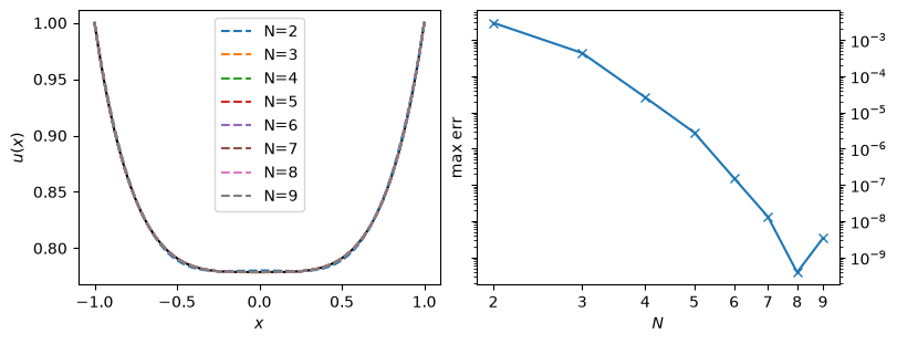
The right plot shows the absolute errors on a log-log plot.
Why do the errors bottom out at \(\sim 10^{-9}\)?
How do the errors scale as a function of the number of basis functions?
Solution
This is because
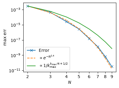
scipy.optimize.curve_fit()callsscipy.optimize.least_squares(), which has a default tolerance of \(10^{-8}\). Increasing the tolerance gives the plot in the margin.Playing a bit, you can find that the absolute error behaves like
\[\begin{gather*} \epsilon \sim e^{-N^{1.4}}. \end{gather*}\]I doubt this has an significance, but it does capture the behavior over the shown range.
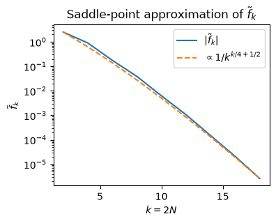
To gain a better understanding, note that the Chebyshev basis is really a Fourier basis in disguise. Thus, the convergence is determined by the asymptotic behaviour of the Fourier transform of
\[\begin{gather*} f(\theta) \sim u(x) \sim e^{\cos^4\theta}, \qquad x = \cos\theta. \end{gather*}\]This can be estimated using the saddle-point approximation. Let \(x_0 = \cos\theta_0\):
\[\begin{gather*} \tilde{f}_{k} = \int_{0}^{2\pi} e^{-\I k \theta + \cos^4\theta}\d{\theta} \approx \pm \I e^{-\I k \theta_0 + x_0^4} \sqrt{\frac{2\pi}{4x_0^2(3 - 4x_0^2)}} \end{gather*}\]where \(\theta_0\) is a saddle-point of the integrand:
\[\begin{gather*} 0 = \diff{(-\I k \theta_0 + \cos^4\theta_0)}{\theta_0} = -\I k - 4\cos^3\theta_0\sin\theta_0 \\ = -\I k - 4x_0^3\sqrt{1-x_0^2}. \end{gather*}\]There is a saddle-point on the negative imaginary axis \(\theta_0 = -\I b\) where
\[\begin{gather*} k = 4\cosh^3{b} \sinh{b} \approx \frac{e^{4b}}{4}, \qquad b \approx \frac{\ln 4k}{4},\\ -\I k\theta_0 \approx \frac{- k\ln 4k}{4}, \\ x_0 = \cos\theta_0 \approx \cosh b \approx \frac{e^{b}}{2} = \frac{(4k)^{1/4}}{2}, \qquad x_0^4 \approx \frac{k}{4},\\ -\I k \theta_0 + x_0^4 \approx \frac{k(1 - \ln 4k)}{4},\\ \tilde{f}_{k} \sim \frac{1}{k^{k/4+1/2}}. \end{gather*}\]The largest \(k\) in our basis corresponds to \(\cos(2N \theta)\) so \(k_{\max} = 2N\) and the truncation error should be proportional to the missing terms with \(k = 2(N+1)\). This is approximately correct. (See the plots to the right, which verify that the saddle-point approximation is good, but there is some deviation in this scaling – the basis is slightly better than expected.)
Best Pseudo-Spectral Fit#
For the Chebyshev polynomials, the collocation points are the roots of the \(T_{N}(x)\), in other words, where \(\cos(N \cos^{-1} x) = 0\), or \(N\cos^{-1}x = (i + \tfrac{1}{2})\pi\):
In our cases, an \(N\) term solution is built upon \(T_{2n}\) up to \(T_{2N}(x)\). Recall that we skip the odd orders because of the parity of our solution: likewise, we need only keep the positive collocation points:
With these, we can exactly solve for the coefficients \(a_n\) using
numpy.linalg.solve(), minimizing the pseudo-spectral residual to exactly zero:
def get_xi(N):
    """Return the N collocation points."""
    i = np.arange(N)
    xi = np.cos((i + 0.5) * np.pi / 2 / N)
    return xi

def get_a(N, exact=exact):
    x_ = get_xi(N)[:, None]
    n_ = 1 + np.arange(N, dtype=float)[None, :]
    k_ = 2*n_
    A = np.cos(k_*np.arccos(x_)) - 1
    a = np.linalg.solve(A, exact(x_.ravel()) - 1)
    return a
[0.10705744 0.03425387]
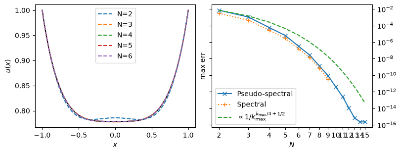
Although the errors are slightly larger than with the spectral method (which directly
minimizes the residual), they still decrease exponentially, and are very comparable, and
code is much simpler (no need to call curve_fit()).
Solving the BVP#
This previous analysis shows how well we might do with (pseudo-)spectral methods, but cheats by using the exact solution. We now apply the method to directly solve the ODE. The only change is that we now use the ODE as our residual:
Note that these equations are inhomogeneous because of our incorporation of the boundary conditions into \(u_{\vect{a}}(x)\):
The only thing we need is the second derivative of the basis functions, which can be computed using the chain rule:
def phi(x, n, d=0):
    """Return the dth derivative of phi_n(x)"""
    th = np.arccos(x)
    cn = np.cos(2*n*th)

    if d == 0:
        return cn - 1

    sn = np.sin(2*n*th)
    s = np.sin(th)

    if d == 1:
        return (2*n) * sn / s

    c = np.cos(th)
    if d == 2:
        return -((2*n)**2 * cn * s - (2*n) * sn * c) / s**3


# Check that these are correct... Don't use x0 = 0.5!
x0 = 0.3
h = 1e-8
n = 3
assert np.allclose((phi(x0+h, n) - phi(x0-h, n))/2/h, phi(x0, n, d=1))
assert np.allclose((phi(x0+h, n, d=1) - phi(x0-h, n, d=1))/2/h, phi(x0, n, d=2))

def get_a(N):
    i = np.arange(N)
    xi = np.cos((i + 0.5) * np.pi / 2 / N)
    phis = np.array([phi(xi, n=n) for n in 1+np.arange(N)])
    d2phis = np.array([phi(xi, n=n, d=2) for n in 1+np.arange(N)])
    rhs = xi**6 + 3*xi**2
    A = np.transpose(d2phis - rhs[None, :]*phis)
    a = np.linalg.solve(A, rhs)
    return a

a2 = get_a(2)
print(a2)
[0.10519309 0.03853519]
fig, (ax, ax1) = plt.subplots(1, 2, figsize=(8, 3), constrained_layout=True)
xdata = np.linspace(-1, 1, 500)
ydata = exact(xdata)
ax.plot(xdata, ydata, '-k')
max_errs_ode = []
Ns = np.arange(2, 16)
for N in Ns:
N = int(N)
a = get_a(N)
max_errs_ode.append((abs(model(xdata, *a) - exact(xdata))).max())
if N > 6:
continue
ax.plot(xdata, model(xdata, *a), '--', label=f"{N=}")
ax.legend(loc='upper center')
ax.set(xlabel="$x$", ylabel="$u(x)$")
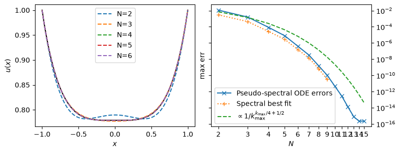
ax1.loglog(Ns, max_errs_ode, '-x', label="Pseudo-spectral ODE errors")
ax1.loglog(Ns[:len(max_errs_spec)], max_errs_spec, ':+', label="Spectral best fit")
k = 2*(Ns+1)
err = 1/k**(k/4 + 0.5)
ax1.loglog(Ns, max_errs_pspec[0]*err/err[0], '--', label=r"$\propto 1/k_{\max}^{k_{\max}/4+1/2}$")
ax1.set(xlabel="$N$", ylabel="max err", xticks=Ns, xticklabels=Ns)
ax1.yaxis.tick_right()
ax1.yaxis.set_ticks_position('both')
ax1.legend(loc="lower left")
a2 = get_a(2)
print(a2)
[0.10519309 0.03853519]