\[\begin{split}
\I\hbar\partial_t
\begin{pmatrix}
\psi_a\\
\psi_b
\end{pmatrix}
=
\begin{pmatrix}
\frac{-\hbar^2 \nabla^2}{2m} + V_a - \mu - \frac{\delta}{2} + g_{aa}n_a + g_{ab}n_b & \frac{\Omega}{2}e^{2\I k_r x} \\
\frac{\Omega}{2}e^{-2\I k_r x} & \frac{-\hbar^2 \nabla^2}{2m} + V_b - \mu + \frac{\delta}{2} + g_{ab}n_a + g_{bb}n_b
\end{pmatrix}
\begin{pmatrix}
\psi_a\\
\psi_b
\end{pmatrix}.
\end{split}\]
Accelerating Frame
We start by considering a primitive transformation to an accelerating frame:
\[\begin{split}
\vect{x} = \vect{x}_v + \vect{x}_0(t), \qquad
\psi'[\vect{x}_v, t] = \psi[\vect{x}_v + \vect{x}_0(t), t], \\
\I\hbar\partial_t \psi'(\vect{x}_v, t) =
\I\hbar\partial_t\psi[x_v + x_0(t), t] +
\I\hbar\dot{\vect{x}}_0(t)\cdot\vect{\nabla}\psi[x_v + x_0(t), t].
\end{split}\]
Gradients are not affected by this transformation, but the time-dependence of the coordinate change induces an additional piece that must be added to the Hamiltonian:
\[
\I\hbar\partial_t \psi'(\vect{x}_v, t) = \Bigl(
\op{H} - \dot{\vect{x}}_0(t)\cdot\vect{\op{p}}
\Bigr)\psi'(\vect{x}_v, t).
\]
This is a valid and practical implementation of the transformation to an accelerating references, but is not the usual form of a Galilean transformation. We present it here as it will correspond to the transformation of type (B) considered below. Now we consider the more conventional transformation which includes the phase modification. We effect a similar transformation as in the previous section:
\[\begin{split}
x = x_v + x_0(t), \qquad
\psi_{v}(x_v, t) = e^{-\I\phi}\psi(x_v + x_0(t), t), \qquad
\hbar\phi = m\dot{x}_0(t)x_v + \int_0^{t}\frac{m\dot{x}_0^2(t)}{2}\d{t},\\
\I\hbar \dot{\psi}_v(x_v, t)
= \left(\frac{-\hbar^2\nabla_v^2}{2m} + V\bigl(x_v + x_0(t)\bigr) + m\ddot{x}_0(t)x_v\right)\psi_v(x_v, t).
\end{split}\]
Here the only difference is that we pick up an additional linear potential corresponding to the fictitious force from the acceleration.
Applying this to the two-component system we have
$$
x_v(t) = x - x_0(t), \qquad
\Psi(x, t) = \exp\left{
\frac{\left[mx_v\dot{x}0(t) + \int_0^{t}\frac{m\dot{x}0^2(t)}{2}\d{t}\right]\mat{1}
- \hbar k_R [x_v + x_0(t)]\mat{\sigma}{z}}{\I\hbar}
\right}
\tilde{\Psi}{v}(x_v, t)\
\I\hbar \dot{\tilde{\Psi}}_{v}(x_v, t)
= \mat{\tilde{H}}v \tilde{\Psi}{v}(x_v, t)\
\mat{\tilde{H}}_v =
(24)\[\begin{pmatrix}
\frac{\hbar^2 (k+k_R)^2}{2m} + V_a\bigl(x_v + x_0(t)\bigr) + mx_v\ddot{x}_0(t) + \hbar k_R \dot{x}_0(t) & \frac{\Omega}{2}\\
\frac{\Omega}{2} & \frac{\hbar^2 (k-k_R)^2}{2m} + V_b\bigl(x_v + x_0(t)\bigr) + mx_v\ddot{x}_0(t) - \hbar k_R \dot{x}_0(t)
\end{pmatrix}.
$$
+++
### Moving Bucket/Detuning Ramp Equivalence.
+++
From the previous discussion, we see that modulating the detuning $\delta(t)$ with potentials $V[x]$ is equivalent to moving to a different frame with velocity $\dot{x}_0(t) = [\delta(0) - \delta_v(t)]/2\hbar k_R$ with effective potentials $V[x_v + x_0(t)] + mx_v \ddot{x}_0(t)$. If the potential is harmonic $V(x) = m\omega^2x^2/2$, then:
+++
$$
V[x_v + x_0(t)] + m x_v \ddot{x}_0(t) =
\frac{m\omega^2}{2}[x_v + x_0(t)]^2 + m[x_v + x_0(t)] \ddot{x}_0(t) - m x_0(t) \ddot{x}_0(t) =
\frac{m\omega^2}{2}\left[
x_v + x_0(t) + \frac{\ddot{x}_0(t)}{\omega^2}
\right]^2 - \frac{m\ddot{x}^2_0(t)}{2\omega^2} - m x_0(t) \ddot{x}_0(t)
$$
+++
Reversing this, suppose we have a harmonic potential moving with position $y_0(t)$ so that in the lab frame, the system has $V[x - y_0(t)]$. We can cancel the effect of this motion boosting to a frame with position $x_0(t)$ such that
$$
x_0(t) + \frac{\ddot{x}_0(t)}{\omega^2} = y_0(t).
$$
Similarly, this system can be simulated by manipulating the detuning as:
$$
\delta(t) = \delta_0 - 2\hbar k_R \dot{x}_0(t).
$$
+++
### Classical Transformation
+++
#### (L) Lab Frame: $H(x, p)$
+++
It will be useful to consider the classical analogue for the motion of the center of mass of the cloud. To do this, we formulate the classical problem with an arbitrary dispersion:
$$
H(x, p) = E_d[p] + V[x].
$$
We shall call this the "Lab Frame" (L), and the dispersion here may have some detuning $d$.
+++
#### (A) Moving Frame A: $H_v(x_v, p_v)$
+++
It is useful to consider this system in a moving frame with coordinate $x_v = x - x_0(t)$ which can be effected using the following generating function $G(p_v, x)$ for a Canonical transform:
$$
G(p_v, x) = p_v[x - x_0(t)] + m x \dot{x}_0(t), \\
x_v = \pdiff{G}{p_v} = x - x_0(t), \qquad
p = \pdiff{G}{x} = p_v + m\dot{x}_0(t),\\
H'(x_v, p_v) = H + \pdiff{G}{t}
= E_d[p_v + m \dot{x}_0(t)] - p_v\dot{x}_0(t) + V[x_v + x_0(t)] + m [x_v + x_0(t)] \ddot{x}_0(t),
$$
The form of this transform is fixed by the condition that $x_v = x - x_0(t)$ and the condition that one usually wants $p_v = p - m\dot{x_0}(t)$.
*Note: The latter condition refers to some mass $m$ which has no meaning in the general problem. Thus a better approach may be to simply take $G(p_v, x) = p_v[x - x_0(t)]$ in which case $p_v = p$ is the momentum in the lab frame. We consider this below for frame (B). This is consistent with the general problem which does not display Galilean covariance. However, we will be comparing with a system that has Galilean covariance in which $m$ is defined, so we use the augmented transform here.*
+++
Now we consider a harmonic potential $V(x) = m\omega^2x^2/2$. In this case we find the following Hamiltonian in the moving frame:
$$
H_v(x_v, p_v) = E_d[p_v + m \dot{x}_0(t)] - p_v\dot{x}_0(t)
+ \frac{m\omega^2}{2}\left[x_v + x_0(t) + \frac{\ddot{x}_0(t)}{\omega^2}\right]^2
- \frac{m\ddot{x}_0^2(t)}{2\omega^2}.
$$
+++
Now, if we choose $\delta(t) = 2\hbar k_R\dot{x}_0(t)$ and express this in dimensionless coordinates with units of $\hbar = k_R = 2E_R = 1$ so that $d = \delta/4E_R$, then we have:
$$
d = \dot{\tilde{x}}_0, \qquad
y_0(t) = x_0(t) + \frac{\ddot{x}_0(t)}{\omega^2},\\
\tilde{H}_{v}(\tilde{x}_v, \tilde{k}_v) =
\tilde{E}_d(\tilde{k}_v + d) - \tilde{k}_vd + \frac{\tilde{\omega}^2}{2}[\tilde{x}_v + \tilde{y}_0(t)]^2 - \text{const}
= \tilde{E}_{0}(\tilde{k}_v) + \frac{\tilde{\omega}^2}{2}[\tilde{x}_v + \tilde{y}_0(t)]^2 - \text{const}.
$$
+++
Here we note that the boosted dispersion $\tilde{E}_d(\tilde{k}_v + d) - \tilde{k}_vd = \tilde{E}_0(\tilde{k}_v) + \text{const}$. In other-words, by boosting to a frame with $\dot{x}_0=\delta(t)/2\hbar k_R$, we have removed the effects of the detuning:
$$
E_{d}(k+d) - kd = \frac{(k+d)^2+1}{2} \pm \sqrt{(k+d-d)^2+w^2} - kd\\
= \frac{k^2+1}{2} \pm \sqrt{k^2+w^2} + \frac{d^2}{2}
= E_{0}(k) + \frac{d^2}{2}.
$$
Thus:
$$
E_{d}(k+d) = E_{0}(k) + kd + \frac{d^2}{2}, \quad
E_{d}(k) = E_{0}(k-d) + kd - \frac{d^2}{2}\\
$$
+++
We shall refer to this transformation as Moving Frame (A): $H_v(x_v, p_v)$.
+++
#### (B) Moving Frame: $H_v'(x_v, p)$
+++
An alternative canonical transformation is to drop the $mx\dot{x}_0(t)$ piece from the generator $G(p_v, x)$:
$$
G(p_v, x) = p_v[x - x_0(t)], \qquad
x_v = x - x_0(t), \qquad p_v = p, \qquad
H'_v(x_v, p) = E_d[p] - p\dot{x}(t) + V[x_v + x_0(t)].
$$
We shall refer to this transformation as Moving Frame (B): $H'_v(x_v, p)$.
+++
### Summary
+++
#### Lab Frame (L)
$$
H(x, k)=E_d(k)+V(x),\\
\dot{x} = E_d'(k), \qquad
\dot{k} = -V'(x).
$$
#### Moving Frame (A)
$$
x_v = x - x_0, \qquad
k_v = k - m\dot{x}_0\\
H_v(x_v, k_v) = E_0(k_v) + V(x_v + x_0) + (x_v + x_0) \ddot{x}_0,\\
\dot{x}_v = E_0'(k_v), \qquad
\dot{k}_v = -V'(x_v + x_0) - \ddot{x}_0.
$$
#### Moving Frame (B)
$$
x_v = x - x_0, \qquad
k_v = k,\\
H_v'(x_v, k) = E_d(k) - k\dot{x}_0 + V(x_v + x_0),\\
\dot{x}_v = E_d'(k) - \dot{x}_0, \qquad
\dot{k} = -V'(x_v + x_0).
$$
+++
### Stationary Solutions
+++
*(To simplify the notations, we drop the tildes here: everything is dimensionless.)*
To test this, we consider the stationary solution or ground state at finite $d$ in the lab frame. This has momentum $k=k_0$ such that $E'_{d}(k_0) = 0$. Here are the corresponding solutions in the three frames:
| Lab Frame (L) | Moving Frame (A) | Moving Frame (B) |
|---------------------------|-------------------------------|-----------------------------------------|
| $H(x, k)=E_d(k)+V(x)$ | $H_v(x_v,k_v)=E_0(k_v)+V(x_v+dt)$ | $H'_v(x_v,k) = E_d(k) - kd + V(x_v+dt)$ |
| $x=0$ | $x_v = x - dt$ | $x_v = x - dt$ |
| $k=k_0$ | $k_v = k_0 - d$ | $k = k_0$ |
| $\dot{x}=E_d'(k_0)=0$ | $\dot{x}_v=E_0'(k_v)=-d$ | $\dot{x}_v=E'_d(k_0)-d$ |
| $\dot{k}=-V'(0)=0$ | $\dot{k}_v=-V'(x_v-dt)=0$ | $\dot{k}_v=-V'(x_v-dt)=0$ |
We have used $E_0'(k_v) = E_d'(k_v+d)-d = -d$.
+++
# Trapping Potentials
+++
The physical trapping potential is from intersecting lasers with a roughly Gaussian shape. If the cloud is small, this can be well approximated by a Harmonic Trap, but for larger clouds (i.e. the axial direction in the experiments) the Gaussian shape becomes important, so we include that here.
$$
I = \frac{2 P}{\pi w^2}e^{-2(y^2+z^2)/w^2}, \qquad
w = w_0\sqrt{1+\frac{x^2}{x_R^2}}, \qquad
x_R = \pi \frac{w_0^2}{\lambda}, \\
$$
This is described by the following physical parameters:
* $w_0 = $20μm: Central beam waist.
* $\lambda = $1064nm: Frequency of laser.
* $P = $???: Power of the laser.
Near the center, we obtain the following harmonic potential (assuming $V = -A\pi I/2P$):
$$
V_{HO} = \frac{-2A}{\pi w_0^2} + \frac{m}{2}\Bigl(\omega_x^2x^2 + \omega_\perp^2(y^2+z^2)\Bigr), \qquad
\omega_\perp^2 = \frac{4 A}{m w_0^4}, \qquad
\omega_x^2 = \frac{2A\lambda^2}{m\pi^2w_0^6}.
$$
As a check, the ratio of the trapping frequencies is
$$
\frac{\omega_\perp}{\omega_x} = \sqrt{2}\pi \frac{w_0}{\lambda} \approx 83.52.
$$
This slightly disagrees with the trapping frequencies listed before:
$$
\frac{\nu_\perp}{\nu_x} = \frac{287\mathrm{Hz}}{3.07\mathrm{Hz}} = 90.55.
$$
To be consistent, we use the previous relationship in the code to specify $w_0$ and the coefficient $A$ in terms of the trapping frequencies as follows:
$$
w_0 = \frac{\omega_\perp}{\omega_x}\frac{\lambda}{\sqrt{2}\pi}, \qquad
A = \frac{m w_0^4 \omega_\perp^2}{4}, \qquad
x_R = \pi \frac{w_0^2}{\lambda},\qquad
w = w_0\sqrt{1+\frac{x^2}{x_R^2}}, \\
V_{\mathrm{ext}}(x, y, z) = A\left(\frac{1}{w_0^2} - \frac{e^{-2(y^2+z^2)/w^2}}{w^2}\right).
$$
```{code-cell}
import sympy
```
```{code-cell}
sympy.init_session(quiet=True)
m, w_0, lam, A, Ap, epsilon, w_x, w_perp, x, y, z = sympy.symbols(
"m w_0 lambda A P epsilon \\omega_x \\omega_\\perp x y z".split(" ")
)
x_R = sympy.pi * w_0**2 / lam
w = w_0 * sympy.sqrt(1 + x**2 / x_R**2)
I = 2 * P / sympy.pi / w**2 * sympy.exp(-2 * (y**2 + z**2) / w**2)
V_ = -sympy.pi * A / 2 / P * I
display(V_)
```
```{code-cell}
w_0_ = w_perp / w_x * lam / sympy.sqrt(2) / sympy.pi
A_ = m * w_0_**4 * w_perp**2 / 4
V = V_.subs({A: A_, w_0: w_0_})
V_HO = sympy.expand(
sympy.series(V.subs(dict(x=epsilon * x, y=epsilon * y, z=epsilon * z)), epsilon, n=3)
.removeO()
.subs(epsilon, 1)
)
V_HO_perp = sympy.expand(
sympy.series(V.subs(dict(x=x, y=epsilon * y, z=epsilon * z)), epsilon, n=3)
.removeO()
.subs(epsilon, 1)
)
V, V_HO, V_HO_perp
```
```{code-cell}
%pylab inline
from gpe.soc import u
x_TF = 234.6 * u.micron
w_x = 2 * np.pi * 2.07 * u.Hz
w_perp = 2 * np.pi * 278 * u.Hz
r_TF = x_TF * np.sqrt(w_x / w_perp)
lam = 1064 * u.nm
w_0 = w_perp / w_x * lam / np.sqrt(2) / np.pi
A = -u.m * w_0**4 * w_perp**2 / 4
x_R = np.pi * w_0**2 / lam
x = np.linspace(-x_TF, x_TF)[:, None]
r = np.linspace(0, r_TF)[None, :]
y = z = 0
w = w_0 * np.sqrt(1 + (x / x_R) ** 2)
V = A * (np.exp(-2 * (r**2) / w**2) / w**2 - 1 / w_0**2)
V_HO = u.m * ((w_x * x) ** 2 + (w_perp * r) ** 2) / 2
plt.subplot(211)
plt.plot(x, (V[:, 0] / V_HO[:, 0] - 1))
# plt.plot(x, (V[:, -1]/V_HO[:, -1] - 1))
plt.xlabel("x")
plt.ylabel("rel err in V")
plt.subplot(212)
_n = x.shape[0] // 2
# plt.plot(r[0,:], (V[_n, :]/V_HO[_n, :] - 1))
plt.plot(r[0, :], V[_n, :])
plt.plot(r[0, :], V_HO[_n, :], ":")
np.sqrt(2) * np.pi * (20 * 1000) / 1064, 278 / 3.07
```
# Using the Code
+++
We start with a simple demonstration. Here we start from a flat background and imprint a bump which we subsequently let expand. For this purpose, we use the `soc.ExperimentBarrier` class as a base, specifying the depth, position, width of the barrier. The various `soc.State*` classes will delegate to this experiment class to compute the potentials as a function of time. This allows the same experiment to be studied using a variety of states (1D, tube, axial, one-component vs two-component etc.)
+++
## Initial State
+++
The initial state should be specified in terms of `V_TF` which is used in the Thomas Fermi approximation to determine the initial state. Alternatively one can specify `x_TF` where `V_TF = V_ext(x_TF)` however there are some subtleties with this approach that make the second option a bit more complicated.
The experiments are designed to be contained within a harmonic trap with frequencies `experiment.trapping_frequencies_Hz`. The initial state is specified through the parameter `x_TF` which specifies where the initial cloud should end assuming that it is well approximated by the Thomas-Fermi approximation (i.e. the healing length is small compared with the features of the trapping potentials such as the barrier). Since the initial state preparation must be tailored to the experiment, we rely on `Experiment.get_state()` rather than `State.set_initial_state()` as was described in [BEC.ipynb](BEC.ipynb) and [`bec.py`](../gpe/bec.py). Here is the basic protocol:
```python
Experiment.set_state():
# <choose State class and basis>
state = State()
V_TF = self.fiducial_V_TF # Memoizes self.get_fiducial_V_TF()
state.set_initial_state(V_TF):
ns = self.get_ns_TF(V_TF)
<define phases>
self.data[...] = phases*np.sqrt(ns)
```
The actual generation of an initial state is not quite so simple to allow for two additional use cases. These factors go into determining the fiducial `V_TF`:
1. **`expt`**: We wish to generate small states that focus on the central portion of a larger trap. These states will often not contain any abscissa at `x_TF`, so the procedure used in `get_Vs_TF()` will fail or be grossly inaccurate. The `expt=True` flag means we should compute things in the original large experimental trap with the original experimental trap frequencies `ws_expt`.
2. **`fiducial`**: In the experimental case of cooling in the presence of a bucket, one often starts with an `x_TF` specified *without* the bucket, thus the potential used to determine `V_TF` will need to ignore the time-dependent (bucket) portion of the potential. The `fiducial=True` flag means that we should compute things in the initial experimental setup where `x_TF` has meaning, which may have a different initial potential which is later adiabatically turned on to prepare the true initial state. The initial ground state should then have the same *particle number* as the initial fiducial state, but this will required a different `V_TF`.
These case are enabled by the `get_fiducial_V_TF()` of `Experiment` class in [`soc.py`](../gpe/soc.py). See its docstring for a detailed explanation. It calls the following functions of the `Experiment` class with the additional boolean arguments `expt` and `fiducial` allowing subclasses to customize the preparation of the initial state:
* `Experiment.get_Vext(state, fiducial=False, expt=False)`: If `expt=True`, then `ws_expt` should be used for the trap. (This allows one to set, e.g. `w_x=0` when looking for phonons on a homogeneous background near the center of a large trap.) If `fiducial=True` is used, then a different initial potential might be used – i.e. without the bucket – which should match the semantic meaning of `x_TF`.
* `State.set_initial_state(V_TF, fiducial=False, expt=False)`: This generally should just pass the appropriate parameters to `experiment.get_Vext()`.
```{code-cell}
import gpe.imports
```
```{code-cell}
reload(gpe.imports)
from gpe.imports import *
```
```{code-cell}
from SOC import soc_catch_and_release
```
```{code-cell}
e = soc_catch_and_release.ExperimentCatchAndReleaseSmall()
s = e.get_state()
```
```{code-cell}
from gpe import soc
from gpe.soc import u
class Experiment(soc.ExperimentBarrier):
B_gradient_mG_cm = 0
barrier_depth = 0.0
barrier_width = 1.0 * u.micron
barrier_x = 0.0
def barrier_depth_t_(self, t_):
if t_ <= 0:
return self.barrier_depth
else:
return 0.0
experiment = Experiment(Lx=40 * u.micron, Nx=256, x_TF=10 * u.micron)
s0 = experiment.get_state()
s0.plot()
# s = experiment.get_initial_state()
# Va, Vb, Vab = s0.get_Vext()
# x = s0.xyz[0].ravel()
# plt.plot(x, Va, x, Vb)
```
```{code-cell}
s0.plot()
m = MinimizeState(s0)
m.check()
s = m.minimize(psi_tol=1e-6)
s.plot()
```
```{code-cell}
e = EvolverABM(s, dt=0.4 * s.t_scale, normalize=True)
with NoInterrupt() as interrupted:
while e.t < 10 * u.ms and not interrupted:
e.evolve(10)
plt.clf()
e.y.plot()
display(plt.gcf())
clear_output(wait=True)
```
# Homogeneous States and the Bloch Sphere
In the rotating phase basis, we can consider homogeneous states:
$$
\tilde{\Psi} = e^{\I k x}
\begin{pmatrix}
\sqrt{n_a}\\
\sqrt{n_b}
\end{pmatrix}.
$$
(*States with a different relative momentum will develop density oscillations.*) We can neglect the evolution of this overall phase by subtracting an appropriate constant chemical potential to obtain the following rotation on the Bloch sphere:
$$
\tilde{\Psi} = \exp\left(-\I t \vec{\omega}\cdot \frac{\vec{\mat{\sigma}}}{2}\right)\tilde{\Psi}, \qquad
\vec{\omega} = \begin{pmatrix}
\frac{\Omega}{\hbar}\\
0\\
\frac{2\hbar k k_r}{m} - \frac{\delta}{\hbar}
\end{pmatrix}.
$$
Recall:
$$
\mat{\sigma}_i \cdot\mat\sigma_{j} = \delta_{ij}\mat{1} + \I\epsilon_{ijk}\mat{\sigma}_{k}, \qquad
\Tr\mat{\sigma}_{i}\cdot\mat{\sigma}_{j} = 2\delta_{ij}, \\
\mat{\sigma}_i \cdot\mat\sigma_{j}\cdot\mat\sigma_{k}
= \I e_{ijk}\mat{1} + (d_{ij}s_k - d_{ik}s_j + d_{jk}s_i) \qquad
\mat{\sigma}_i \cdot\mat\sigma_{j}\cdot\mat\sigma_{k}\cdot\mat\sigma_{l}
= (d_{ij}d_{kl} - d_{il}d_{jk} + d_{ik}d_{jl})\mat{1}
+ \I (d_{ij}e_{lkn} + d_{lk}e_{ijn} - d_{ln}e_{ijk} + d_{kn}e_{ijl})\mat{\sigma}_n\\
\Tr(\mat{\sigma}_i \cdot\mat\sigma_{j}\cdot\mat\sigma_{k}) = 2\I e_{ijk}, \qquad
\Tr(\mat{\sigma}_i \cdot\mat\sigma_{j}\cdot\mat\sigma_{k}\cdot\mat\sigma_{l})
= 2(d_{ij}d_{kl} - d_{il}d_{jk} + d_{ik}d_{jl})
$$
To parameterize the state itself it is useful to use the density matrix:
$$
\mat{\rho} = \ket{\tilde{\Psi}}\bra{\tilde{\Psi}}
= \frac{1}{2}\left(\mat{1} + \vec{a}\cdot\vec{\mat{\sigma}}\right).
$$
One can then check that the vector $\vec{a}\rightarrow\vec{a}'$ rotates as a vector in SO(3).
$$
a'_i = \frac{a_j}{2}\Tr\left[\mat{\sigma}_{i}\cdot
\exp\left(-\I t \vec{\omega}\cdot \frac{\vec{\mat{\sigma}}}{2}\right)
\cdot\mat{\sigma}_j
\cdot\exp\left(\I t \vec{\omega}\cdot \frac{\vec{\mat{\sigma}}}{2}\right)
\right], \qquad
\vec{a}' = e^{t\vec{\omega}\times}\cdot\vec{a}.
$$
+++
In dimensionless units:
$$
\frac{\omega}{4E_R} = \begin{pmatrix}
w\\
0\\
1 - d
\end{pmatrix}\]
\[ \begin{align}\begin{aligned}```{code-cell}
import numpy as np
from scipy.linalg import expm
from gpe.utils import pauli_matrices, levi_civita\\np.random.random
np.random.seed(1)
a = np.random.random(3)
a /= np.linalg.norm(a)
wt = np.random.random(3) * 0.1\\one = np.eye(2)\\
def get_rho(a):
return (one + np.einsum("a, aij->ij", a, pauli_matrices)) / 2.0\\
L2 = np.einsum("a,aij->ij", wt, -1j * pauli_matrices / 2.0)
L3 = np.einsum("a,aij->ij", wt, -levi_civita[3])
U2 = expm(L2)
U3 = expm(L3)\\rho = U2.dot(get_rho(a)).dot(U2.T.conj())
rho1 = get_rho(U3.dot(a))
assert np.allclose(rho, rho1)
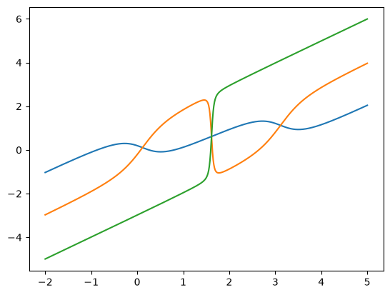
```\\## Homogeneous Phases\\```{code-cell}
%pylab inline --no-import-all
k = np.linspace(-5, 5, 1000)
d = -1.0
w = 0.5 / 4
D = np.sqrt((k - d) ** 2 + w**2)
plt.plot(k, (k**2 + 1) / 2.0 - D)
plt.plot(k, (k**2 + 1) / 2.0 + D)
```\\# Linear Response (Bogoliubov Theory)\\+++\\## Single Component\\:::{margin}
Sometimes the equations developed here are referred to as the Bogoliubov-de Gennes (BdG)
equations because they look similar to the equations from superconducting theory. See
{cite}`Fetter:2009` for details.
:::
For homogeneous states we can perform a Bogoliubov analysis of the small amplitude modes. We start with the GPE for a single component, but with arbitrary dispersion. This will be appropriate, for example, if the lower branch of the dispersion is occupied:\end{aligned}\end{align} \]
\I\hbar\dot{\Psi} = H[n]\Psi = \left(E_-(\op{p}) + gn\right)\Psi, \qquad
H[n]\Psi = \frac{\delta E[\Psi]}{\delta \Psi^\dagger}
$$
which follows from minimizing the following energy functional:
\[
E[\Psi] = \int \left(
\Psi^\dagger E_-(\op{p})\Psi + \frac{g}{2}(\Psi^\dagger\Psi)^2
\right)\d{x}.
\]
Consider the following homogeneous solution of the GPE:
\[
\Psi_k(x,t) = \sqrt{n}e^{\I (kx - \omega_k t)}, \qquad
\hbar\omega_k = E_-(k) + gn.
\]
Note that this might not be the ground state if \(k \neq k_0\) which minimizes \(E_-(k)\), but is a homogeneous solution of the time-dependent GPE. It represents the ground state boosted to a frame with phase velocity \(k-k_0\) and group velocity \(v = E_-'(k)\).
To this, we add a small perturbation of order \(\delta\) so that the wavefunction has the form:
\[
\Psi = \Psi_k + \delta \Psi_1.
\]
Furthermore, we restrict the perturbation so that it does not change the total particle number (to order \(\delta\)) which requires that \(\Psi_1\) be orthononal to \(\Psi_k\):
\[
\int \Psi_1^\dagger \Psi_k \d{x} = 0.
\]
(Alternatively, we can drop this restriction, and then include the chemical potential \(\mu = \hbar \omega_k = E_{k} + gn\) explicitly in the Hamiltonian \(\op{H}\).) The energy of this new state will be
\[\begin{split}
E[\Psi] - E[\Psi_0]
= \delta\Psi_1^\dagger \frac{\delta E[\Psi]}{\delta \Psi^\dagger} + \text{h.c.}
= \delta\Psi_1^\dagger \op{H}[n]\Psi + \text{h.c.}\\
= \delta\Psi_1^\dagger \op{H}[n](\Psi_k + \delta\Psi_1) + \text{h.c.}\\
\end{split}\]
\[
\Psi(x,t) = e^{\I kx}\left(\sqrt{n} + \delta (u e^{\I(qx - \omega t)}
+ v^* e^{-\I(qx-\omega t)})\right).
\]
This represents two plane waves of magnitude \(\sim \delta\) with wave-vector \(q\) and frequency \(\omega\). The Bogoliubov equations express the relationship between \(\omega\) and \(k\) in order for this to be a solution of the GPE to order \(\delta\) (dropping order \(\delta^2\) and higher terms).
Once we solve this, the energy-density of the perturbed state will be:
\[
\mathcal{E} = \I\hbar \frac{\int\left( \Psi^\dagger E_-(\op{p})\Psi + \frac{gn^2}{2}\right) \d{x}}{V}
=
\hbar\delta^2 \omega
\left(
(u^* e^{-\I(qx - \omega t)} + v e^{\I(qx-\omega t)})
(u e^{\I(qx - \omega t)} - v^* e^{-\I(qx-\omega t)})
\right)
=
\hbar\delta^2 \omega\left(\abs{u}^2 - \abs{v}^2\right)
\]
with a small perturbation of order \(\delta\) with momentum \(q\) and frequency \(\omega\) on top of a background state of homogeneous density \(n\) and wave-vector \(k\). This gives rise to the following normal modes:
\[\begin{split}
\begin{pmatrix}
E(k+q) - E(k) + gn - \omega & gn\\
gn & E(k-q) - E(k) + gn + \omega
\end{pmatrix}
\cdot
\begin{pmatrix}
u \\
v
\end{pmatrix} =
\begin{pmatrix}
A - \omega & D\\
D & B + \omega
\end{pmatrix}
\cdot
\begin{pmatrix}
u \\
v
\end{pmatrix} = 0.
\end{split}\]
The spectrum is given by:
\[\begin{split}
-AB + (B-A)\omega + \omega^2 + D^2 = 0, \qquad
\omega = \frac{A-B}{2} \pm \sqrt{\frac{(A+B)^2}{4} - D^2},\\
\omega = E_- \pm \sqrt{E_+(E_+ + 2gn)}, \qquad
E_{-} = \frac{E(k+q) - E(k-q)}{2}, \qquad
E_{+} = \frac{E(k-q) + E(k+q) - 2E(k)}{2}.
\end{split}\]
\[\begin{split}
\begin{pmatrix}
A & D\\
D & B
\end{pmatrix}
\begin{pmatrix}
u\\
v
\end{pmatrix}
=
\omega
\begin{pmatrix}
1 & 0\\
0 & -1
\end{pmatrix}
\begin{pmatrix}
u\\
v
\end{pmatrix}
\end{split}\]
The sign of the overall energy is given by the expression
\[\begin{split}
\begin{pmatrix}
u^* & v^*
\end{pmatrix}
\begin{pmatrix}
A & D\\
D & B
\end{pmatrix}
\begin{pmatrix}
u\\
v
\end{pmatrix}
=
\omega (\abs{u}^2 - \abs{v}^2)
\end{split}\]
The eigenvalues of this matrix are:
\[
E_+ \pm \sqrt{E_-^2 + D^2}
\]
hence the condition for energetic stability is that \(E_+ > - \sqrt{E_-^2+D^2}\).
In the ground state of the lower band, we have
\[\begin{split}
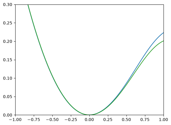
E(k) = E_0 + \frac{(k-k_0)^2}{2m^*} + C (k-k_0)^3 + \order(k-k_0)^4\\
\frac{1}{m^*} = E''(k_0), \qquad
C = \frac{E'''(k_0)}{3!}.
\end{split}\]
The Bogoliubov spectrum about \(k=k_0\) then simplifies to:
\[
\omega = \pm cq\left(1 + \frac{q^2}{2m_*}\frac{1}{4m_*c^2}\right) + C q^3 + \order(q^5), \qquad
c = \sqrt{\frac{gn}{m_*}}, \qquad
\]
\[\begin{split}
E(k) = \frac{k^2+1}{2} - D, \qquad
D = \sqrt{(k-d)^2 + w^2}\\
E'(k) = k - K(k), \qquad
K(k) = D'(k) = \frac{k-d}{D}\\
E''(k) = 1 - K'(k) = 1 - \frac{w^2}{D^3}\\
E'''(k) = 3\frac{w^2(k-d)}{D^5} = 3\frac{w^2}{D^4}K(k)\\
\end{split}\]
In the ground state, \(K(k_0) = k_0\) and \(D_0 = D(k_0) = (k_0-d)/k_0\), so
\[\begin{split}
E''(k_0) = \frac{1}{m_*} = 1 - \frac{w^2}{D_0^3}\\
E'''(k_0) = C = 3\frac{w^2k_0}{D_0^4}
= \frac{3}{D_0}\left(1 - \frac{1}{m_*}\right)\\
\end{split}\]