Getting Started with the GPE

We start with an example of a 1D quantum gas in a periodic potential. In the next document Getting Started in Higher Dimensions, we explore higher dimensions

For our purposes, we consider the following model for a dilute Bose-Einstein condensate (BEC) of neutral \({}^{78}\)Rb atoms in a 1D periodic potential with the Gross-Pitaevski equation (GPE):

\[\begin{gather*} \I\hbar \dot{\psi} = \left(\frac{-\hbar^2 \nabla^2}{2m} + V(x, t) - \mu + g n\right), \qquad n = \abs{\psi}^2. \end{gather*}\]

Dimensions/Units

I remember these as follows:

\[\begin{gather*} [\hbar] = ET,\\ N = \int n\d^{d}x,\\ [gn = \mu] = E,\\ [\tfrac{1}{2}mv^2] = E. \end{gather*}\]

We start by a simple dimensional analysis

\[\begin{gather*} [\hbar] = \frac{ML^2}{T}, \qquad [n] = \frac{1}{L^{d}}, \qquad [\psi] = \frac{1}{L^{d/2}}, \qquad [\mu] = \frac{ML^2}{T^2}, \qquad [g] = \frac{ML^{2+d}}{T^2}. \end{gather*}\]

To derive others, we note that \(\hbar/m\) and \(g/m\) are independent of mass. These can then be combined to find length and time scales:

\[\begin{gather*} \left[\frac{(\hbar/m)^{2}}{g/m}=\frac{\hbar^2}{mg}\right]^{\frac{1}{2-d}} = L, \qquad \left[\frac{(\hbar/m)^{2+d}}{(g/m)^{2}}\right]^{\frac{1}{2-d}} = T. \end{gather*}\]

Note that this fails in \(d=2\) dimensions and that the 2D GPE famously has a scaling symmetries.

Details

We start with

\[\begin{gather*} \left[\frac{(\hbar/m)^{a}}{(g/m)^{b}}\right] = L^{2a-(2+d)b}T^{2b-a}. \end{gather*}\]

For distance, we want

\[\begin{gather*} 2a-(2+d)b = 1, \qquad 2b-a = 0\\ a = 2b, \qquad b = \frac{1}{2-d}, \qquad a = \frac{2}{2-d}. \end{gather*}\]

For time, we want

\[\begin{gather*} 2a-(2+d)b = 0, \qquad 2b-a = 1\\ a = 2b-1, \qquad b = \frac{2}{2 - d}, \qquad a = \frac{2+d}{2 - d} \end{gather*}\]

Scaling in 2D

In 2D, we have

\[\begin{gather*} [\hbar/m] = \frac{D^2}{T}, \qquad [g/m] = \left(\frac{D^2}{T}\right)^2. \end{gather*}\]

Thus, we cannot use these to define a distance and length scale. This manifests as an explicit scaling symmetry for solution. To see this, note that if we have a solution \(\psi(\vect{x}, t)\), then the following is also a solution for all \(s\):

\[\begin{gather*} \psi_s(\vect{x}, t) = \frac{1}{s}\psi(s\vect{x}, s^2t). \end{gather*}\]

The key point is that, under this scaling of dimensions, all terms in the GPE scale the same way by a factor of \(1/s^2\). The overall scaling of \(\psi_s\) follows from its dimensions, which must be \([\psi] = 1/D\) so that the particle number remains fixed:

\[\begin{gather*} \int \d^2{\vect{x}}\abs{\psi_s(s\vect{x})}^2 = N. \end{gather*}\]

As you get more comfortable with these types of problems, you might be able to skip this step and directly code something – or create some classes with sensible defaults. For now, we are explicit.

Before implementing something numerically, we should determine the scales in our problem. We start with a theory perspective: the relevant length scales for this system are:

• Density \(n\): The length-scale here is the interparticle spacing, the relation of which to density depends on dimension. In 1D, we have \([n] = 1/L\). This is often expressed in terms of the interparticle spacing \(n^{-1/d}\) where \(d\) is the dimension.

  It is common to use \(\xi = h\) to represent the healing length (e.g. [Pethick and Smith, 2002]), but we reserve this usage for the Bertsch parameter describing the unitary Fermi gas (UFG). We will never use \(h\) to represent \(2\pi \hbar\) in these notes.

• Healing length \(h\): This is the length scale over which the gas will go from the background density \(n_0 = \mu/g\) to zero and represents a balance between the kinetic energy and the non-linear interactions:

  \[\begin{gather*} \frac{\hbar^2}{2mh^2} \approx \mu = gn_0, \qquad h = \sqrt{\frac{\hbar^2}{2m\mu}}= \frac{\hbar}{\sqrt{2m g n_0}}. \end{gather*}\]

  It might be tempting to try to relate the speed of sound and healing length

  \[\begin{gather*} h = \frac{\hbar}{\sqrt{2}mc} \end{gather*}\]

  but as we discuss in the box, this depends on the specific form of the equation of state \(\mathcal{E}(n)\).

• Speed of Sound \(c\): Related to these is the speed of sound. This can be calculated by looking at the Phonon Dispersion from the Linear Response of a homogeneous system to small perturbations:

  \[\begin{gather*} c = \sqrt{\frac{gn_0}{m}}. \end{gather*}\]

Equation of State \(\mathcal{E}(n)\).

we have presented everything here for the GPE which models a system with energy density

\[\begin{gather*} \mathcal{E}(n) = \frac{E}{V} = \frac{g}{2} n^2. \end{gather*}\]

More generally, we might consider a system that has a different equation of state, and related thermodynamic properties like the chemical potential \(\mu\), pressure \(p\), and the (isoentropic) compressibility \(\kappa\). These are related as follows from standard thermodynamics:

\[\begin{gather*} \mu = \mathcal{E}'(n), \qquad p = \mu n - \mathcal{E}(n), \qquad c^2 = \frac{p'(n)}{m} = \frac{n\mathcal{E}''(n)}{m} = \frac{1}{mn\kappa}. \end{gather*}\]

In terms of the equation of state, we thus have

\[\begin{gather*} h = \sqrt{\frac{\hbar^2}{2m\mathcal{E}'(n)}}, \qquad c^2 = \frac{n\mathcal{E}''(n)}{m}. \end{gather*}\]

In this sense, the healing length and speed of sound are fundamentally different quantities, and the relationship between the two depends on the nature of the system.

The density \(n\) and healing length \(h\) are intrinsic properties of the system. They represent physics and we must choose relevant scales here. To simulate systems numerically, we must consider some additional length scales:

Independence of the box size is called IR-convergence.

• Box size \(L_x\): This represents the extent of our system and is sometimes called the infrared- or IR-scale* since we cannot simulate features with wavelengths longer than this. Note: this might be physical if we have a trapped gas, where the box size must be larger than the size of the trapped cloud. However, it might also be a numerical artifact when studying homogeneous or periodic systems where we would really like to know what happens in the IR limit (a.k.a. thermodynamics limit) \(L_x \rightarrow \infty\).

  Independence of the lattice spacing is called UV-convergence.

• Lattice spacing \(\d{x}\): This represents the smallest feature we can resolve in our system, sometimes called the ultraviolet- or UV-scale since we cannot simulate features with wavelengths smaller than this. This is almost never physical, and instead represents a numerical limitation. We almost always want to know what the results are in the UV-limit \(\d{x} \rightarrow 0\).

To reliably simulate physics with our numerical implementation of the GPE we need:

Diluteness is typically expressed in terms of the s-wave scattering length \(a\), which, in 3D, is related to the coupling constant by

\[\begin{gather*} g = \frac{4\pi \hbar^2 a}{m}, \qquad na^{3} \ll 1. \end{gather*}\]

We can re-express this in terms of the ratio of the healing length \(h\) to the interparticle spacing \(n^{-1/d}\):

\[\begin{gather*} \frac{n^{-1/d}}{h} = \sqrt{8\pi an^{1/d}} \ll 1. \end{gather*}\]

1. Spatial resolution (UV convergence): The lattice spacing must be smaller than the healing length. When using spectral methods, it often suffices to have \(\d{x}\) a few times smaller. For finite-difference methods, UV convergence is much more difficult to obtain.

   \[\begin{gather*} \d{x} < h. \end{gather*}\]

2. IR convergence: The box must be big enough to contain the relevant physics. Together, these set the cost of our simulation – we need \(N_x \geq L_x/\d{x}\) lattice points.

3. Diluteness: This is not explicitly built into the previous parameters, but the GPE is not valid if the interactions are too strong or if the range of the interaction \(r_0\) is too large. Formally, we must have both

   \[\begin{gather*} r_0 \ll n^{-1/d} \ll h. \end{gather*}\]

   If the healing length is comparable to the interparticle spacing, then there will be an appreciable non-condensed fraction that must be considered, while if the effective range is too large, then the interaction terms \(gn\) must be modified to include three-body interactions etc.

We could work entirely in dimensionless units, and you will see this in the literature (see the box). To facilitate later comparison with experiments, we will set our units in terms of the convenient parameters \(m_{^{87}Rb} \approx 87\)u, \(\hbar\), and microns μm = m\(^{-6}\). In principle, we could include the 3D scattering length for rubidium, but this will get rolled into the 1D coupling constant with parameters like the transverse trapping frequency, so we will not fix this for now.

Do It! Canonical Form of the GPE

The GPE can be scaled into a canonical form often seen in the mathematics literature

\[\begin{gather*} \I u_{,t} = -\tfrac{1}{2}u_{,xx} + \sigma \abs{u}^2u + \tilde{V}u, \qquad \sigma = \pm 1. \end{gather*}\]

This is equivalent to choosing a system of units such that \(\hbar = m = g = 1\) so that

\[\begin{gather*} 1 = \underbrace{m}_{\text{mass}} = \underbrace{\left(\frac{\hbar^2}{mg}\right)^{1/(2-d)}}_{\text{distance}} = \underbrace{\left(\frac{(\hbar/m)^{2(2+d)}}{(g/m)^{4}}\right)^{1/(2-d)}}_{\text{time}}, \end{gather*}\]

but be careful: this does not work in \(d=2\) which has an additional scale invariance. Alternatively, one can change variables:

\[\begin{gather*} \tilde{x} = \frac{x}{a}, \qquad \tilde{t} = \frac{t}{b}, \qquad \tilde{V} = \frac{V}{c}, \qquad u = \frac{\psi}{f}, \qquad \end{gather*}\]

(Find appropriate constants \(a\), \(b\), \(c\), and \(f\).) One cannot scale away the sign of the interactions. Attractive interactions \(\sigma = -1\) are called focusing while repulsive interactions \(\sigma = 1\) (as we deal with here) are called defocusing. In some of the mathematical literature, you will see this referred to as the (de)focusing non-linear Schrödinger equation (NLSEQ). Various authors might also choose a scaling that absorbs the factor of 2, or includes it with \(\sigma\), and use the acronym (NLS) or (NLSE), so be careful to check the definitions. (Rarely, authors might also change the sign of \(\I\)…)

Question to ponder: What happens to dimensionless parameters such as the diluteness parameter \(an^{1/d}\)?

Note: if the potential is flat \(V(x) = \mu = \) const., then the 1D GPE is integrable, admitting and infinite set of conserved quantities, such as the particle number \(N\), energy \(E\), momentum \(P\), etc. In the dimensionless form, these are related to the constants \(C_i\) defined in Eq.(37) of [Zakharov and Shabat, 1972]:

\[\begin{gather*} 2\I C_1 = \frac{-\sigma}{2} \int \abs{u}^2 \d{x} \propto \frac{-\sigma}{2}N\\ (2\I)^2 C_2 = \frac{\sigma}{4} \int (u^*u_{,x} - u u^*_{,x}) \d{x} \propto \frac{\I\sigma}{2}P\\ (2\I)^3 C_3 = \frac{\sigma}{2} \int \left(\abs{u_{,x}^2} + \frac{\sigma}{2}\abs{u}^4\right) \d{x} \propto \frac{\sigma}{2}E\\ (2\I)^4 C_4 = \frac{-\sigma}{2} \int \left(uu^*_{,xxx} - 3\frac{\sigma}{2}uu_{,x}^*\abs{u}^2\right) \d{x}. \end{gather*}\]

The first three constants follow from symmetries and Noether’s theorem: \(U(1)\) phase invariance, translation invariance, and time-translation invariance respectively. The rest are a consequence of the integrability.

To enable us to play, we allow the user to set the physical parameters:

• healing_length_micron: The healing length \(h\) in microns (micrometers μm = m\(^{-6}\)).

• dx_healing_length: The lattice spacing in units of the healing length.

• Lx_microns: The box size in microns.

• n0_micron: The background/central density in units of inverse microns.

From these, and physical constants such as the particles mass \(m\) and \(\hbar\), we can fix the other physical parameters, such as the chemical potential, and coupling constant.

\[\begin{gather*} \mu = \frac{\hbar^2}{2mh^2}, \qquad g = \frac{\mu}{n_0}. \end{gather*}\]

Defining a Problem

To set up a simulation, we must create a State class that implements the gpe.interfaces.IStateGPE interface. Here we define all the parameters in a subclass. We will also include an external potential, which we will take to be a (periodic) gaussian

\[\begin{gather*} V(x) \approx V_0 \exp\left(-\frac{x^2}{2\sigma^2}\right), \end{gather*}\]

which introduces two new parameters

• V0_mu: \(V_0\) expressed in units of the chemical potential \(\mu\).

• sigma_healing_length: \(\sigma\) expressed in units of the healing length.

Coding Conventions

After some years of experience working with Python code, we have established some coding conventions.

1. Unless you have an explicit reason not to, follow PEP-8.

2. Use [Black][] to format your code. This minimizes redundant changes in spaceing, etc. so that version control has less noise and remains useful for exploring significant changes. It also frees developers from agonizing about formatting, improving coding speed.

3. Most of our code is aimed at high performance in longer simulations. This often requires some 2initialization, precomputing quantities that will be reused etc. before running long simulations. Traditionally, such initialization is done in the contructor (__init__() in Python), but we would also like to enable users to be able to change attributes or parameters of their simulations after construction. The standard approach is to use getters and setters (@property in Python) but dealing with dependencies becomes a chore (i.e. if you change one parameter, you might need update another). After exploring many options, I have landed on a solution that works well for our needs:

   The constructor sets all attributes with minor checks (types, conversion to arrays etc.), then calls init() which performs any initializations needed to get the class ready for simulation. The init() method will also be called by pre_evolve_hook() and pre_minimize_hook() – part of the intefaces – before simulations/minimization start, allowing changed parameters to be properly considered.

4. We currently provide *_GPU methods that are used in the core simulation loops. These return GPU arrays (or other forms of acceleration) and have matching CPU methods get_Vext() which wrap these and transfer the GPU arrays to the CPU for plotting. (Such transfers are expensive, and should be avoided in the simulations loops.) GPU methods should be carefully designed to allow both CPU and GPU usage for performance. This means that self.xp should be used in place of np for example and that all arrays should be assumed to be GPU arrays.

5. Our current recommendation is to use the State to describe the type of system – i.e. Bosons or Fermions with particular interactions or dispersions – and then use an Experiment class which implements gpe.interfaces.IExperiment to define the experimental parameters – how is the state prepared, measured, etc.

   For simplicity, we first define a stand-along state class, then we generalize.

import numpy as np
import matplotlib.pyplot as plt

from gpe.bec import StateGPEBase, u
from gpe.utils import get_good_N


class State(StateGPEBase):
    healing_length_micron = 1.0 # Healing length in microns
    dx_healing_length = 0.5     # Maximum lattice spacing in units of the healing length
    Lx_micron = 10.0            # Box length in units of microns
    V0_mu = -1.0                # Depth of the potential in units of the chemical potential.
    sigma_healing_length = 1.0  # Width of the potential in healing lengths
    n0_micron = 1.0             # Background density
    
    def __init__(self, **kw):
        for key in list(kw):
            if hasattr(self, key):
                setattr(self, key, kw.pop(key))

        m = u.m_Rb87
        hbar = u.hbar
        self.healing_length = self.healing_length_micron * u.micron
        Lx = self.Lx_micron * u.micron
        dx = self.dx_healing_length * self.healing_length
        n0 = self.n0_micron / u.micron
        
        # Select a good Nx that will perform well - small prime factors.
        Nx = get_good_N(Lx / dx)

        # Calculate the chemical potential and g
        mu = hbar**2 / 2 / m / self.healing_length
        g = mu / n0
        kw.update(hbar=hbar, m=m, Lxyz=(Lx,), Nxyz=(Nx,), mu=mu, g=g)
        super().__init__(**kw)

    def init(self):
        """Perform any initializations before the simulation begins."""
        # Units
        self.V0 = self.V0_mu * self.mu
        self.sigma = self.sigma_healing_length * self.healing_length
        super().init()

    def get_Vext(self):
        x, = self.get_xyz()
        V_ext = self.V0 * np.exp(-(x/self.sigma)**2/2)
        return V_ext 

s = State()
s.plot();

/home/docs/checkouts/readthedocs.org/user_builds/gpe/conda/latest/lib/python3.14/site-packages/gpe/utils.py:2755: PerformanceWarning: Default State.get_Vext_GPU() delegates to non-GPU version.

This is a potential performance issue, even if not using the GPU.  To ensure optimal
performance, you should make sure that you overload get_Vext_GPU() instead.

  warnings.warn(

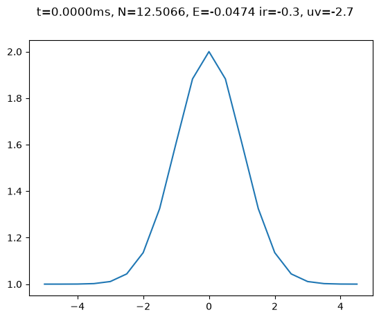
The state is populated using the Thomas-Fermi approximation

\[\begin{gather*} n_{TF}(x) = \frac{\mu - V(x)}{g}. \end{gather*}\]

We can evolve this and see how close we are to the ground state of the system. Since we want to explore the dynamics, we code this in a function:

from pytimeode.evolvers import EvolverABM
from mmfutils.contexts import FPS

def plot_states(states):
    # Always plot dimensionless quantities...
    t_unit = u.ms
    x_unit = u.micron
    n_unit = 1 / x_unit

    plot_Nlr = hasattr(states[0], 'get_Nlr')
    
    s = states[-1]
    ns = np.array([s.get_density() for s in states])
    Es = np.array([s.get_energy() for s in states])
    Ns = np.array([s.get_N() for s in states])
    if plot_Nlr:
        Nlr = np.transpose([s.get_Nlr() for s in states])
    ts = np.array([s.t for s in states])
    xs = np.ravel(s.xyz[0])

    kw = dict(sharex=True,  gridspec_kw=dict(hspace=0))
    if plot_Nlr:
        fig, axs = plt.subplots(3, 1, height_ratios=(0.2, 0.5, 1), **kw)
    else:
        fig, axs = plt.subplots(2, 1, height_ratios=(0.2, 1), **kw)

    ax = axs[0]
    E, N = Es[0], Ns[0]
    ax.plot(ts / t_unit, Es / E - 1, label="$E$")
    ax.plot(ts / t_unit, Ns / N - 1, label="$N$")
    ax.set(ylabel="Rel. change", title=f"{E=:.4g}, {N=:.4g}")
    ax.legend()

    if plot_Nlr:
        ax = axs[1]
        Nl, Nr = Nlr
        ax.plot(ts / t_unit, Nl/Nl[0] - 1, label="$N_l$")
        ax.plot(ts / t_unit, Nr/Nl[0] - 1, label="$N_r$")
        ax.set(ylabel="Rel. change in $N_{lr}$")
        ax.legend()

    ax = axs[-1]
    mesh = ax.pcolormesh(ts / t_unit, xs / x_unit, ns.T / n_unit)

    # Label your axes...
    ax.set(ylabel="$x$ [μm]", xlabel="$t$ [ms]")

    # ... and your colorbars.
    fig.colorbar(mesh, ax=axs.ravel().tolist(), label="$n$ [1/μm]")


def evolve(s, T_ms=20, Nt=200, dt_t_scale=0.4, timeout_s=60):
    """Evolve the state s to time T and plot.
    
    Arguments
    ---------
    s : State
        Initial state.
    T_ms : float
        Final time in ms.
    Nt : int
        Number of frames to plot.
    dt_t_scale : float
        Step size for evolve in units of t_scale = hbar/maximum resolvable energy.
    timeout_s : float
         Timeout (in seconds).
    """
    T = T_ms * u.ms
    dT = T / Nt

    # Note: From experience, if you have chosen dx correctly, you should
    # get highly converged results if you use a time-step dt between 0.2 and 0.5 times
    # s.t_scale.  If you can go much larger, you are probably wasting effort.  If need
    # to go much smaller, you probably have an incorrect lattice spacing.
    dt = dt_t_scale*s.t_scale
    
    # Make sure we can take integer steps...
    steps = max(int(np.ceil(dT / dt)), 2)
    dt = dT / steps
    
    ev = EvolverABM(s, dt=dt)
    states = [ev.get_y()]
    for frame in FPS(frames=Nt, timeout=timeout_s):
        ev.evolve(steps)
        states.append(ev.get_y())


    plot_states(states)
    return states

states = evolve(s)

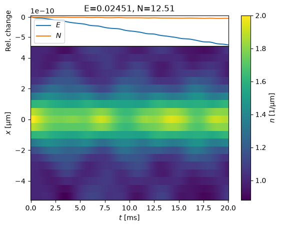
We see some fluctuations, but overall the energy \(E\) and particle number \(N\) are conserved to 9 digits. Here is what might happen if we choose too large of a time-step:

evolve(s, dt_t_scale=1.0);

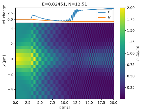
The energy is not conserved here: going larger, the code might crash with ABM.

Minimization

To get a high-quality initial state, we can run a minimizer:

Notice that the scales have 1e-15 on the top left. The first means that the relative change in energy and particle number is \(\lesssim \pm 2.5\times 10^{-15}\).

from gpe.minimize import MinimizeState

s0 = State()
s = MinimizeState(s0, fix_N=False).minimize(use_scipy=True)
evolve(s);

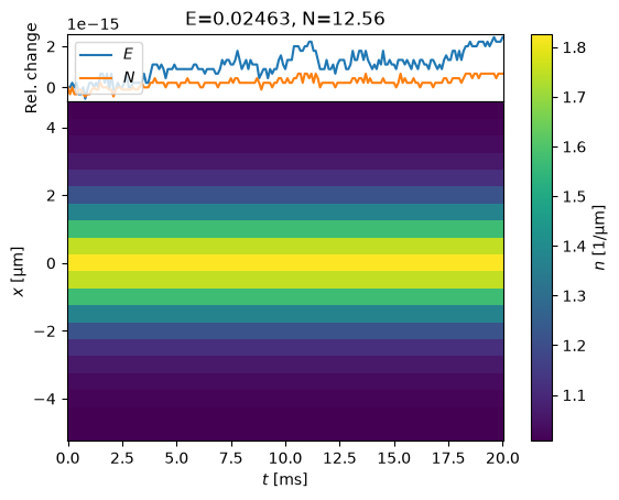
Now the state is static to high precision – the fluctuations that you see are on the order of \(10^{-15}\).

Josephson Oscillations

Stationary states are pretty boring. Let’s do something more exciting. Here we consider inducing real-space Josephson oscillations as follows:

This is done with an attractive laser. The profile is gaussian, but close to the center we can approximate this with a quadratic potential.

1. Place the atoms in a harmonic trap. This needs a new parameter, the trap frequency \(\omega_x\):

   \[\begin{gather*} V_{HO}(x) = \frac{m\omega_x^2x^2}{2}. \end{gather*}\]

2. Find the ground state with a repulsive barrier \(V_0 < 0\).

This is done with a magnetic field gradient.

3. Jump on a linear potential. For a harmonic oscillator, this simply shifts the location of the minimum, so instead, we just use

   \[\begin{gather*} V_{HO}(x) = \frac{m\omega_x^2(x-x_0)^2}{2}. \end{gather*}\]

What do you think will happen?

For \(^{87}\)Rb, we have

\[\begin{gather*} m\approx 87\text{u}, \qquad a\approx 100 a_B \approx 5\text{nm}. \end{gather*}\]

Parameters

If you are familiar with experiments, you might know what good trap frequencies are, and for a particular species, you can find the mass \(m\) and coupling constant

\[\begin{gather*} g = \frac{4\pi \hbar^2 a_s}{m} \end{gather*}\]

where \(a_s\) is the S-wave scattering length. Otherwise, it might be better to specify the Thomas-Fermi radius of the trap \(x_{TF}\) where

\[\begin{gather*} \frac{m\omega_x^2x_{TF}^2}{2} = \mu, \qquad \omega_x = \frac{\sqrt{2\mu/m}}{x_{TF}}. \end{gather*}\]

If we then choose a scale for the central density \(n_0 = g\mu\), this fixes the coupling constant, trap frequencies, etc.

class StateJosephson(State):
    x_TF_micron = 50.0
    x0_micron = 20.0
    Lx_micron = 200.0   # Need bigger box
    V0_mu = 2.0         # Repulsive barrier
    
    def init(self):
        """Perform any initializations before the simulation begins."""
        # Units
        self.x0 = self.x0_micron * u.micron
        x_TF = self.x_TF_micron * u.micron
        self.wx = np.sqrt(2*self.mu/self.m)/x_TF
        super().init()
    
    def get_Nlr(self):
        """Return the number of particles on the left and right respectively."""
        x, = self.xyz
        n = self.get_density()
        N = self.integrate(np.where(x<0, 1, 1j) * n)
        Nl, Nr = N.real, N.imag
        return Nl, Nr

    def get_Vext(self):
        x, = self.get_xyz()
        
        V_ext = super().get_Vext()
        if (self.initializing or self.t < 0):
            x0 = 0.0
        else:
            x0 = self.x0
        V_ext += self.m * (self.wx*(x-x0))**2/2
        return V_ext

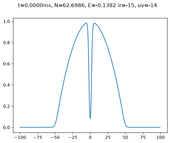
s0 = StateJosephson()
%time s = MinimizeState(s0, fix_N=False).minimize()
s.plot()

CPU times: user 1e+03 ms, sys: 5.95 ms, total: 1.01 s
Wall time: 554 ms

/home/docs/checkouts/readthedocs.org/user_builds/gpe/conda/latest/lib/python3.14/site-packages/gpe/utils.py:2755: PerformanceWarning: Default StateJosephson.get_Vext_GPU() delegates to non-GPU version.

This is a potential performance issue, even if not using the GPU.  To ensure optimal
performance, you should make sure that you overload get_Vext_GPU() instead.

  warnings.warn(

[<Axes: >]

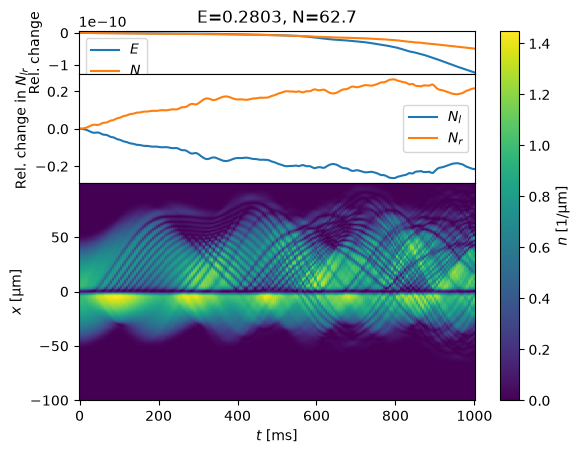
%time evolve(s, T_ms=1000);

CPU times: user 21 s, sys: 186 ms, total: 21.2 s
Wall time: 10.7 s

s0 = StateJosephson(V0_mu=4.0)
%time s = MinimizeState(s0, fix_N=False).minimize()
%time evolve(s, T_ms=1000);

CPU times: user 562 ms, sys: 0 ns, total: 562 ms
Wall time: 282 ms
CPU times: user 21.2 s, sys: 177 ms, total: 21.4 s
Wall time: 10.7 s

This is fun, but I think we are mixing several different bits of the physics. I suggest you now take the time to review the Josephson effect.

The Josephson Effect

The essence of the Josephson effect is a current

\[\begin{gather*} I = I_c \sin \phi_{-}, \qquad \dot \phi_{-} = \frac{2\delta V}{\hbar}, \end{gather*}\]

where \(\phi_{-} = \phi_R - \phi_L\) is the phase difference between the BECs on the right and left of the barrier.

DC Josephson Effect

To generate a DC current, we simply imprint the desired phase difference \(\phi_-\) on the initial state:

class StateJosephsonDC(StateJosephson):
    x0_micron = 0.0  # No shift now
    dphi = np.pi/2   # Josephson phase difference.

    def initialize_state(self):
        self.t = 0
        s = MinimizeState(self, fix_N=False).minimize(use_scipy=True)
        x = s.xyz[0]
        phi_x = self.dphi / 2 * np.sign(x)
        psi = np.sqrt(s.get_density()) * np.exp(1j*phi_x)
        self.set_psi(psi)

s = StateJosephsonDC()
%time s.initialize_state()
%time states = evolve(s, T_ms=200)

CPU times: user 819 ms, sys: 984 μs, total: 820 ms
Wall time: 412 ms
CPU times: user 5.16 s, sys: 29 ms, total: 5.19 s
Wall time: 2.62 s

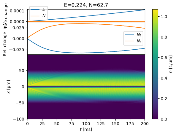
Notice that we start with a constant DC current. After some time, however, this current causes a density difference on either side. The mean-field interaction therefore induces a potential difference \(\delta V \approx g \delta n\) that eventually changes the phase, arresting and reversing the flow.

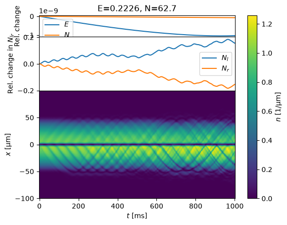
AC Josephson Effect

If we instead fix a potential difference difference \(\delta V\), then the phase will wind, generating an alternating current:

class StateJosephsonAC(StateJosephson):
    x0_micron = 0.0     # No shift now
    dV_mu = 0.2         # Josephson "voltage" difference 
    
    def init(self):
        self.x0 = self.x0_micron * u.micron
        x_TF = self.x_TF_micron * u.micron
        self.wx = np.sqrt(2*self.mu/self.m)/x_TF
        self.dV = self.dV_mu * self.mu
        super().init()
    
    def get_Vext(self):
        x, = self.get_xyz()
        
        V_ext = super().get_Vext()
        if (self.initializing or self.t < 0):
            pass
        else:
            V_ext += self.dV * np.sign(x)
        return V_ext
    

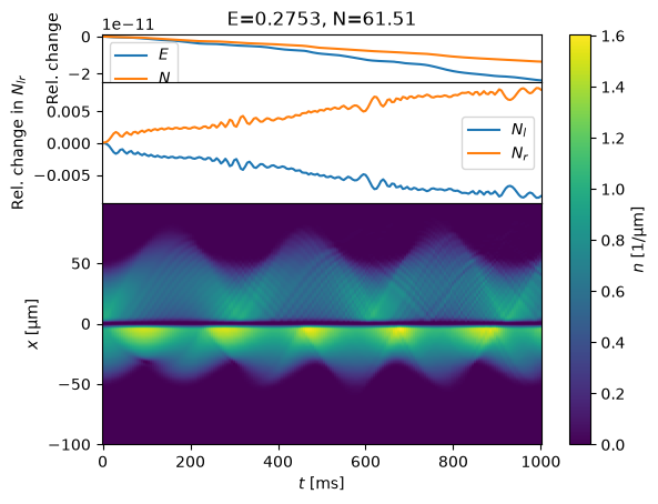
s0 = StateJosephsonAC()
%time s = MinimizeState(s0, fix_N=False).minimize(use_scipy=True)
%time states=evolve(s, T_ms=1000)

CPU times: user 744 ms, sys: 0 ns, total: 744 ms
Wall time: 375 ms
CPU times: user 21.6 s, sys: 213 ms, total: 21.8 s
Wall time: 11 s

/home/docs/checkouts/readthedocs.org/user_builds/gpe/conda/latest/lib/python3.14/site-packages/gpe/utils.py:2755: PerformanceWarning: Default StateJosephsonAC.get_Vext_GPU() delegates to non-GPU version.

This is a potential performance issue, even if not using the GPU.  To ensure optimal
performance, you should make sure that you overload get_Vext_GPU() instead.

  warnings.warn(

Do it!

Is this the appropriate/expected DC Josephson effect? Check that the corresponding frequencies match. Try playing with the parameters – does the Josephson current respond appropriately?

Note: you might see some deviations from the Josephson formulae. Where might these come from? E.g. what role does the trap play? What about the non-linear interactions? How could you adjust your simulation to test for and minimize these effects?

Finally, how can you adjust the parameters to maximize the signal?