Viscosity Notes 5

Viscosity Notes 5#

These are some supporting notes for the document Effective Viscosity.

Microscopic Navier-Stokes#

To better understand the physics of the Navier-Stokes equations, consider representing the gas with a ball-and-“spring” model with \(N+1\) positions \(q_j\) and velocities \(\dot{q}_j\) and inter-particle potential \(V(\delta q)\). In the absence of dissipation we have the Lagrangian

\[\begin{gather*} L[\vect{q}, \dot{\vect{q}}] = \sum_{i=0}^{N} \frac{m}{2}\dot{q}_i^2 - \sum_{i=0}^{N-1} V(q_{i+1} - q_{j}). \end{gather*}\]

The corresponding Euler-Lagrange equations are

\[\begin{gather*} m\ddot{q}_{i} = V'(q_{i+1} - q_{i}) - V'(q_{i} - q_{i-1}) = V'(\delta q_{i}) - V'(\delta q_{i-1}). \end{gather*}\]

To interpret this as a fluid, we introduce the mass density.

\[\begin{gather*} \rho_i = \frac{m}{q_{i+1} - q_{i}} = \frac{m}{\delta q_{i}}. \end{gather*}\]

In the continuum limit the density (and velocity \(u = \dot{q}_i\)) must remain fixed so \(m \sim \delta q_i \rightarrow 0\) in the same way. We can thus write

\[\begin{gather*} \delta q_{i} = \frac{m}{\rho_i}, \qquad \ddot{q}_{i} = \frac{V'(\delta q_{i}) - V'(\delta q_{i-1})}{\rho_i \delta q_i}. \end{gather*}\]

To take the continuum limit, we use the following notation

\[\begin{gather*} f_{i} - f_{i-1} \equiv \delta f \rightarrow \diff{f}{i} = \diff{f}{q}\diff{q}{i} \equiv \delta q \diff{f}{q}. \end{gather*}\]

Thus, the primary tool for effecting this limit are

\[\begin{gather*} \delta \rightarrow \diff{}{i} = \delta q \diff{}{q} = \frac{1}{n}\diff{}{q}, \qquad \delta q \rightarrow \frac{1}{n}\diff{q}{q} = \frac{1}{n}. \end{gather*}\]

Thus:

\[\begin{gather*} \ddot{q}_{i} = \frac{1}{\rho_i \delta q_i}\delta V'(\delta q_i) \rightarrow \frac{1}{m} \frac{1}{n}\underbrace{\diff{V'(1/n)}{q}} _{V''(1/n)\frac{n_{,x}}{n^2}} = V''(1/n)\frac{n_{,x}}{mn^3} = -\frac{n_{,x}}{m}\mathcal{E}''(n), \end{gather*}\]

Thus, in the continuum limit, we must have

\[\begin{gather*} V''(1/n) \sim n^3 \mathcal{E}''(n). \end{gather*}\]

E.g., for the GPE, we have \(\mathcal{E}(n) = gn^2/2\), so \(\mathcal{E}''(n) = g\). Here we set \(r=\delta q = 1/n\) for notational convenience:

\[\begin{gather*} V''(r) = \frac{g}{r^3},\qquad V'(r) = a - \frac{g}{2r^2},\qquad V(r) = \frac{g}{2r} + ar + c. \end{gather*}\]

This means that

\[\begin{gather*} \ddot{q} = \frac{-m\rho_{,x}}{\rho^3} (g n^3) = \frac{-m\rho_{,x}}{\rho^3} \frac{g \rho^3}{m^3} = \frac{-g}{m^2}\rho_{,x}. \end{gather*}\]

Everything here must be finite in the continuum limit, so we must fixed \(g/m^2\) as our interaction strength in order to compare with GPE simulations.

Important

If you are used to working with the GPE, you might naturally think of \(n\) as being finite, but this is because we usually work with a fixed particle mass \(m\) that is already very small. When taking he continuum limit here, you must regard the mass density \(\rho = mn\) as fixed to get the correct scaling.

Strategy for taking the Continuum Limit

My strategy for taking the continuum limit is to express everything in terms of what will become physical quantities:

\[\begin{align*} \rho(x_i) &\sim \rho_i, \\ \rho_{,x}(x_i) &\sim \frac{\rho_{i+1} - \rho_{i}}{q_{i+1} - q_{i}} = \frac{\rho_{i+1} - \rho_{i}}{\delta q_{i+1}}. \end{align*}\]

It is helpful to think of our goal to match the Euler equation

\[\begin{gather*} \ddot{q} = \frac{-\bigl(\mathcal{E}'(n)\bigr)_{,x}}{m} = \frac{-\bigl(\mathcal{E}'(\rho/m)\bigr)_{,x}}{m} = \frac{-\mathcal{E}''(\rho/m)\rho_{,x}}{m^2} = \frac{-\mathcal{E}''(n)n_{,x}}{m}. \end{gather*}\]

Thus, we are trying to manipulate our equations into a form with a gradient:

\[\begin{gather*} \nabla \sim \frac{1}{\delta q_i}. \end{gather*}\]

We must also connect \(\delta q_{i}\) and \(\delta q_{i-1}\):

\[\begin{gather*} \delta q_{i} = \frac{m}{\rho_{i}}, \qquad \rho_{i} \sim \rho_{i-1} + \delta q_{i}\rho_{,x}(x_{i-1}),\\ \delta q_{i-1} = \frac{m}{\rho_{i-1}} = \frac{m}{\rho_{i} - \delta q_{i}\rho_{,x}(x_{i-1})} = \frac{m}{\rho_{i}}\left( 1 + \delta q_{i}\frac{\rho_{,x}(x_{i-1})}{\rho_i} + O(\delta q)^2\right),\\ = \frac{m}{\rho_{i}}\left( 1 + \delta q_{i}\frac{\rho_{,x}}{\rho} + O(\delta q)^2\right). \end{gather*}\]

In the last equation, we note that, since \(\rho_{,x}\) will be finite in the continuum limit, \(\rho_{,x}(x_{i-1}) = \rho_{,x}(x_{i}) + O(\delta q)\), as long as \(\rho_{,xx}\) does not diverge. The key to these manipulations is to keep consistent orders of expansion. We use this to compute

\[\begin{gather*} V'(\delta q_{i-1}) = V'\left( \delta q_i + \delta q_{i}^2\frac{\rho_{,x}}{\rho} + O(\delta q)^3\right),\\ = V'(\delta q_i) + \delta q_{i}^2\frac{\rho_{,x}}{\rho} V''(\delta q_i) + O(\delta q)^3, \end{gather*}\]

from which we can compute the desired result above.

Numerical Check

Here we numerically check this result. We start with \(N\) particles separated such that the initial density is \(n_0(x) \propto R^2-x^2\) where \(R\) is the radius of the initial cloud (Thomas-Fermi radius):

\[\begin{gather*} n(q) = \frac{R^2 - q^2}{\alpha m}, \\ \delta q = q'(i) = \frac{\alpha m}{R^2-q^2}, \\ \int_{-R}^{q} (R^2-q^2)\d{q} = \int_{0}^{i} \alpha m\d{i}, \\ \frac{3q_iR^2 - q_i^3 + 2R^3}{3} = \alpha m i\\ \alpha m = \frac{4R^3}{3N}, \qquad \frac{3\frac{q_i}{R} - \frac{q_i^3}{R^3} + 2}{4} = \frac{i}{N}. \end{gather*}\]

This requires inverting a cubic, which can be done easily using Newton’s method.

One caveat: with these normalizations, we will end up with a fixed mass density \(\rho\), and the number density \(n = \rho/m\) will integrate to the number of particles \(N\). This makes it a little hard to compare things since our physical equation of state \(\mathcal{E}(n) = gn^2/2\) is expressed in terms of the number density. To allow us to compare states with different numbers of particles (i.e., to test the continuum limit), we consider the classical equations:

\[\begin{gather*} \ddot{q} = -\frac{g}{m^2}\rho_{,x} + \cdots. \end{gather*}\]

Thus, we should fix the ratio \(g/m^2\), not \(g\) like we are accustomed to doing with the GPE where \(m\) is held fixed in experiments.

Globally Convergent Newton’s Method

To get our initial density profile, we need to solve

\[\begin{gather*} 3q - q^3 + 2 = (q-2)(q+1)^2 = 4x, \quad q \in [-1, 1], \qquad x \in [0, 1]. \end{gather*}\]

This can be done with Newton’s method, but the current form has zero derivatives at the endpoints, which will cause problems. Using the symmetry of the problem, we restrict ourselves to \(q<0\) and use something linear at the left endpoint:

\[\begin{gather*} f(q) = (q+1) - \sqrt{\frac{4x}{2-q}},\\ f'(q) = 1 - \sqrt{\frac{x}{(2-q)^3}},\\ q_0 = (2x)^{0.6}-1. \end{gather*}\]

This converges to machine precision in 3 steps for all \(x\).

def get_q_R(x, n=3):
    """Return root of 3*q-q**3+2 = 4*x for 0 <= x < 0.5."""
    def f(q, x, d=0):
        if d == 0:
            return q + 1 - np.sqrt(4*x/(2-q))
        elif d == 1:
            return 1 - np.sqrt(x/(2-q)**3)

    def iter(q, x):
        return q - f(q, x) / f(q, x, d=1)
        
    x_ = np.where(x < 0.5, x, 1-x)
    q = (2*x_)**0.6 - 1
    for n in range(n):
        q = iter(q, x_)
    
    return np.where(x < 0.5, q, -q)

x = np.linspace(0, 1)
q = get_q_R(x)
assert abs(3*q - q**3 + 2 - 4*x).max() < 2.1*np.finfo(float).eps

As an additional check, consider the two particles at \(q_{i\pm 1}\) neighboring \(q_{i}\). The net force on the particle at \(q_i\) is

\[\begin{align*} F_{i} &= -V'(q_{i+1}-q_{i}) + V'(q_{i} - q_{i-1}) = -\mathcal{E}''(n)n_{,x},\\ F_{i} &= - V''(\delta q)\diff{\delta q}{i} = - V''(\delta q)\diff{\delta q}{q}\underbrace{\diff{q}{i}}_{\delta q}. \end{align*}\]

Now replacing \(\delta q = 1/n\) we have

\[\begin{gather*} F = - V''(n^{-1})(n^{-1})_{,x}\frac{1}{n} = V''(n^{-1})\frac{n_{,x}}{n^3} = -\mathcal{E}''(n)n_{,x}\\ V''(n^{-1}) = -n^3\mathcal{E}''(n) \end{gather*}\]

Viscosity#

We now model viscosity through a dissipation term in the “springs”. The idea is that there is a resisting force \(F_{\beta}(\delta q, \delta \dot{q})\) that depends on the extension of the spring \(\delta q\) and the velocity \(\delta \dot{q}\):

\[\begin{gather*} F_i = \cdots + \bigl(f(\delta q_{i}, \delta \dot{q}_{i}) - f(\delta q_{i-1}, \delta \dot{q}_{i-1}) = \cdots + \diff{}{i}f(\delta q, \delta \dot{q}),\\ \diff{}{i}f(\delta q, \delta \dot{q}) = \left( f_{,\delta q}\diff{\delta q}{q} + f_{,\delta \dot{q}}\diff{\delta \dot{q}}{q}\right)\diff{q}{i} = \Bigl( f_{,\delta q}(n^{-1})_{,x} + f_{,\delta \dot{q}}(\dot{q}_{,x}n^{-1})_{,x} \Bigr)n^{-1},\\ = -f_{,\delta q}\frac{n_{,x}}{n^3} + f_{,\delta \dot{q}}\left( \frac{\dot{q}_{,xx}}{n^2} - \frac{\dot{q}_{,x}n_{,x}}{n^3} \right) = f_{,\delta \dot{q}}\frac{\dot{q}_{,xx}}{n^2} -(f_{,\delta q} + n\delta \dot{q} f_{,\delta \dot{q}})\frac{n_{,x}}{n^3} \end{gather*}\]

E.g., we can generate a Lamé viscosity:

\[\begin{gather*} \diff{f}{i} = m\nu \frac{(n\dot{q}_{,x})_{,x}}{n}, \qquad f(\delta q, \delta \dot{q}) = m \nu \frac{\delta \dot{q}}{(\delta q)^2}. \end{gather*}\]

Details

I was not sure how to first express this, so I went back to the idea

\[\begin{gather*} \delta q_{i+1} - \delta q_{i} \sim \diff{\delta q}{i} = \diff{\delta q}{q}\diff{q}{i} = \diff{n^{-1} q}{q}\delta q = -\frac{n_{,x}}{n^2}\delta q = -\frac{\rho_{,x}}{\rho}\frac{\delta q}{n} = -\frac{\rho_{,x}}{\rho}\delta q^2. \end{gather*}\]

In other words:

\[\begin{gather*} \delta \sim \diff{}{i} = \diff{q}{i}\diff{}{q} = \delta q\diff{}{q}, \qquad \delta \dot{q} = \delta q \diff{\dot{q}}{q} = \frac{\dot{q}_{,x}}{n}, \end{gather*}\]

etc.

We consider the following two cases:

\[\begin{align*} \frac{\beta f}{m\nu} &\approx \dot{q}_{,xx},\\ \frac{\beta f}{m\nu} &\approx \frac{(n \dot{q}_{,x})_{,x}}{n} = \dot{q}_{,xx} + \frac{n_{,x} \dot{q}_{,x}}{n}. \end{align*}\]

The first is the simple viscosity, while the second is a Lamé viscosity with power \(\alpha = 1\). In both cases:

\[\begin{gather*} \frac{\beta}{m\nu} f_{,\delta \dot{q}} = n^2 = \frac{1}{(\delta q)^2}, \qquad \frac{\beta f}{m\nu} = \frac{\delta \dot{q}}{(\delta q)^2} + g(\delta q). \end{gather*}\]

In the first case, we must have

\[\begin{gather*} f_{,\delta q} + n\delta \dot{q} f_{,\delta\dot{q}} = -2\frac{\delta \dot{q}}{(\delta q)^3} + g'(\delta q) + \frac{\delta \dot{q}}{(\delta q)^3} = g'(\delta q) - \frac{\delta \dot{q}}{(\delta q)^3} = 0,\\ g'(\delta q) = \frac{\delta \dot{q}}{(\delta q)^3}. \end{gather*}\]

This has no solutions since \(g(\delta q)\) should be independent of \(\delta \dot{q}\). In the second case

\[\begin{gather*} \frac{\beta}{m\nu}(f_{,\delta q} + n\delta \dot{q} f_{,\delta\dot{q}}) = -n^2\dot{q}_{,x} = -n^3\delta \dot{q},\\ \frac{\beta}{m\nu}\left( g'(\delta q) - \frac{\delta \dot{q}}{(\delta q)^3} \right) = -\frac{\delta \dot{q}}{(\delta q)^3}, \beta = m \nu, \qquad g(\delta q) = 0. \end{gather*}\]

This is as we stated above.

from scipy.integrate import solve_ivp
from scipy.interpolate import InterpolatedUnivariateSpline

class Particles:
    Ns = 32  # Number of springs
    g_m2 = 1.0  # Coupling constant over mass^2
    R = 1.0  # Initial radius
    beta = 0.0  # Dissipation
    nu = 0.0    # Lame viscosity 
    
    def __init__(self, **kw):
        for key in kw:
            if not hasattr(self, key):
                raise ValueError(f"Unknown {key=}")
            setattr(self, key, kw[key])
        self.init()

    def init(self):
        x0 = np.arange(0, self.Ns+1)/self.Ns
        q0_R = get_q_R(x0)
        self.q0 = self.R * q0_R
        self.m = 4*self.R**3/3/self.Ns
        self.dq0 = 0*self.q0
        self.x0 = np.linspace(-self.R, self.R, self.Ns+1)

    def pack(self, q, dq):
        return np.ravel([q, dq])

    def unpack(self, y):
        return np.reshape(y, (2, y.shape[0]//2) + y.shape[1:])

    def V(self, dq, d=0):
        g = self.g_m2 * self.m**2
        if d == 0:
            return g/2/dq
        elif d == 1:
            return -g/2/dq**2

    def compute_dy_dt(self, t, y):
        q, dq_dt = self.unpack(y)
        dq = np.concatenate([[0], np.diff(q), [0]])
        dV = np.concatenate([[0], self.V(np.diff(q), d=1), [0]])
        ddq_dt = np.concatenate([[0], np.diff(dq_dt), [0]])
        f = self.m * self.nu * ddq_dt/dq**2
        f[0] = f[-1] = 0
        #ddq_dt2 = (dV[1:] - dV[:-1]) / self.m + self.beta * (dv[1:] - dv[:-1])
        ddq_dt2 = (dV[1:] - dV[:-1] + (f[1:] - f[:-1])) / self.m
        return self.pack(dq_dt, ddq_dt2)

p1 = Particles(Ns=32)
p2 = Particles(Ns=256)
ps = [p1, p2]
y0s = [p.pack(p.q0, p.dq0) for p in ps]
T = 2.0
Nt = 100
t_eval = np.linspace(0, T, Nt)
ress = [solve_ivp(p.compute_dy_dt, y0=y0, t_span=(0,T), t_eval=t_eval, method="LSODA")
        for p, y0 in zip(ps, y0s)]
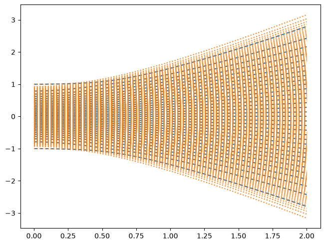
for res, fmt in zip(ress, ['--C0', ':C1']):
    q, dq = p2.unpack(res.y)
    plt.plot(res.t, q.T, fmt);

/tmp/ipykernel_5246/3235063741.py:44: RuntimeWarning: invalid value encountered in divide
  f = self.m * self.nu * ddq_dt/dq**2

../_images/27baa1eee7b3cc46725af4ad5d243a46ab5d13439688e84b512be63deea1d013.png

Nt = len(t_eval)
rhos = []
xs = []
xlim = [0,0]
rho_max = 0
for p, res in zip(ps, ress):
    q, dq = p.unpack(res.y)
    rho = p.m/np.diff(q, axis=0)
    x = (q[1:] + q[:-1])/2
    xlim = [min(xlim[0], x.min()), max(xlim[1], x.max())]
    rho_max = max(rho_max, rho.max())
    rhos.append(rho)
    xs.append(x)
    
args = dict(xlim=xlim, ylim=(0, rho_max))
fig, ax = plt.subplots()
for i in FPS(Nt, fig=fig, embed=True, fps=10):
    ax.cla()
    for j, p in enumerate(ps):
        ax.plot(xs[j][:, i], rhos[j][:, i])
    t = t_eval[i]
    ax.set(title=f"t={res.t[i]:.4f}", **args)

Here is the Lagrangian hydrodynamic description for comparison:

import scipy.fft
sp = scipy

class Flow:
    Nx = 128
    A = 0.5      # g/2/m^2
    nu = 0.04    # Viscosity coefficients

    def __init__(self, **kw):
        for key in kw:
            if not hasattr(self, key):
                raise ValueError(f"Unknown {key=}")
            setattr(self, key, kw[key])
        self.init()
        
    def init(self):
        self._th0 = (2*np.arange(self.Nx) + 1) * np.pi / 2 / self.Nx
        self._k = np.arange(self.Nx)
        self.x0 = np.cos(self._th0)

        # Initial density profile 
        self.n0 = 0*self.x0 + 1.0
        self.n0_x0 = 0*self.x0

        self.n0 = (1-self.x0**2)
        self.n0_x0 = -2*self.x0

    def get_y0(self):
        X0 = self.x0
        Xt0 = 0*X0
        return self.pack(X0, Xt0)
        
    def diff(self, f, d=1):
        ft = sp.fft.dct(f, type=2, norm='forward')
        th, k = self._th0, self._k
        s = np.sin(th)

        # Shift the coefficients and pad with zero.
        df_dth = sp.fft.dst(np.concatenate([-(ft*k)[1:], [0]]), type=3)
        if d == 1:
            df_dx = -df_dth / s
            return df_dx 
        else:
            d2f_dth2 = sp.fft.idct(-ft*k**2, type=2, norm='forward')
            d2f_dx2 = (d2f_dth2 - df_dth / np.tan(th)) / s**2
            if d == 2:
                return d2f_dx2
            return self.diff(df_dx, d=d-2)
    
    def pack(self, X, X_t):
        return np.ravel([X, X_t])

    def unpack(self, y):
        return np.reshape(y, (2, self.Nx))

    def unpack_xnu(self, y):
        X, X_t = self.unpack(y)
        X_x0 = self.diff(X)
        n = self.n0 / X_x0
        u = X_t
        x = X
        return x, n, u

    def get_a_ext(self):
        return 0
        
    def compute_dy_dt(self, t, y):
        X, X_t = self.unpack(y)
        X_x0 = self.diff(X)
        X_x0x0 = self.diff(X, d=2)
        n = self.n0 / X_x0
        n_x = self.n0_x0 / X_x0**2 - self.n0 * X_x0x0 / X_x0**3
        X_tx0 = self.diff(X_t) 
        u_x = X_tx0/X_x0

        u_xx = (self.diff(X_t, d=2)) / X_x0**2 - self.diff(X_t) * X_x0x0 / X_x0**3
        # Zero-laplacian boundary conditions
        u_xx[0] = u_xx[-1] = 0
        
        a_ext = self.get_a_ext()
        X_tt = a_ext - 2*self.A * n_x + self.nu * (n_x * u_x / n + u_xx)
        return self.pack(X_t, X_tt)
        
    def solve(self, T=10.0, Nt=100):
        y0 = self.get_y0()
        t_eval = np.linspace(0, T, Nt)
        res = solve_ivp(self.compute_dy_dt, y0=y0, t_span=(0, T),
                        t_eval=t_eval, method="BDF")
        if not res.success:
            print(res.message)
        self.res = res
        return res

%%time
from scipy.integrate import solve_ivp

p1 = Particles(Ns=32)
p2 = Particles(Ns=256)
ps = [p1, p2]
y0s = [p.pack(p.q0, p.dq0) for p in ps]
T = 2.0
Nt = 100
t_eval = np.linspace(0, T, Nt)
ress = [solve_ivp(p.compute_dy_dt, y0=y0, t_span=(0,T), t_eval=t_eval, method="LSODA")
        for p, y0 in zip(ps, y0s)]
rhos = []
xs = []
xlim = [0,0]
rho_max = 0
for p, res in zip(ps, ress):
    q, dq = p.unpack(res.y)
    rho = p.m/np.diff(q, axis=0)
    x = (q[1:] + q[:-1])/2
    xlim = [min(xlim[0], x.min()), max(xlim[1], x.max())]
    rho_max = max(rho_max, rho.max())
    rhos.append(rho)
    xs.append(x)

f = Flow(A=p1.g_m2/2, nu=0.0)
res = f.solve(T=T, Nt=Nt)
x, n, u = np.einsum('tix->itx', [f.unpack_xnu(y) for y in res.y.T])

args = dict(xlim=(min(xlim[0], x.min()), max(xlim[1], x.max())), 
            ylim=(0, max(rho_max, n.max())))

Nt = len(res.t)
fig, ax = plt.subplots()
for i in FPS(Nt, fig=fig, embed=True, fps=10):
    t = res.t[i]
    ax.cla()
    ax.plot(x[i], n[i], '-')
    for j, p in enumerate(ps):
        ax.plot(xs[j][:, i], rhos[j][:, i], '--')
    t = t_eval[i]
    ax.set(title=f"t={res.t[i]:.4f}", **args)

/tmp/ipykernel_5246/3235063741.py:44: RuntimeWarning: invalid value encountered in divide
  f = self.m * self.nu * ddq_dt/dq**2

CPU times: user 7.49 s, sys: 158 ms, total: 7.64 s
Wall time: 10.5 s

%%time
from scipy.integrate import solve_ivp

nu = 1.0
#p1 = Particles(Ns=32, beta=0.5*32**2)
#p2 = Particles(Ns=256, beta=0.5*256**2)
p1 = Particles(Ns=32, nu=nu)
p2 = Particles(Ns=256, nu=nu)
ps = [p1, p2]
y0s = [p.pack(p.q0, p.dq0) for p in ps]
T = 2.0
Nt = 100
t_eval = np.linspace(0, T, Nt)
ress = [solve_ivp(p.compute_dy_dt, y0=y0, t_span=(0,T), t_eval=t_eval, method="LSODA")
        for p, y0 in zip(ps, y0s)]
rhos = []
xs = []
xlim = [0,0]
rho_max = 0
for p, res in zip(ps, ress):
    q, dq = p.unpack(res.y)
    rho = p.m/np.diff(q, axis=0)
    x = (q[1:] + q[:-1])/2
    xlim = [min(xlim[0], x.min()), max(xlim[1], x.max())]
    rho_max = max(rho_max, rho.max())
    rhos.append(rho)
    xs.append(x)

f = Flow(A=p1.g_m2/2, nu=0.0)
res = f.solve(T=T, Nt=Nt)
x, n, u = np.einsum('tix->itx', [f.unpack_xnu(y) for y in res.y.T])

f = Flow(A=p1.g_m2/2, nu=nu)
res = f.solve(T=T, Nt=Nt)
x, n, u = np.einsum('tix->itx', [f.unpack_xnu(y) for y in res.y.T])

args = dict(xlim=(min(xlim[0], x.min()), max(xlim[1], x.max())), 
            ylim=(0, max(rho_max, n.max())))

Nt = len(res.t)
fig, ax = plt.subplots()
for i in FPS(Nt, fig=fig, embed=True, fps=10):
    t = res.t[i]
    ax.cla()
    ax.plot(x[i], n[i], '-')
    for j, p in enumerate(ps):
        ax.plot(xs[j][:, i], rhos[j][:, i], '--')
    t = t_eval[i]
    ax.set(title=f"t={res.t[i]:.4f}", **args)

/tmp/ipykernel_5246/3235063741.py:44: RuntimeWarning: invalid value encountered in divide
  f = self.m * self.nu * ddq_dt/dq**2

CPU times: user 7.64 s, sys: 96 ms, total: 7.73 s
Wall time: 10.5 s

Viscosity Notes 5

Contents

Viscosity Notes 5#

Microscopic Navier-Stokes#

Viscosity#