Show code cell content

Hide code cell content

import mmf_setup; mmf_setup.nbinit()
import os, sys
from pathlib import Path
FIG_DIR = Path(mmf_setup.ROOT) / '../Docs/_build/figures/'
os.makedirs(FIG_DIR, exist_ok=True)
import logging; logging.getLogger("matplotlib").setLevel(logging.CRITICAL)
%matplotlib
import numpy as np, matplotlib.pyplot as plt
try: from myst_nb import glue
except: glue = None

from matplotlib.animation import FuncAnimation
from gpe.contexts import FPS

$\newcommand{\vect}[1]{\mathbf{#1}} \newcommand{\uvect}[1]{\hat{#1}} \newcommand{\abs}[1]{\lvert#1\rvert} \newcommand{\norm}[1]{\lVert#1\rVert} \newcommand{\I}{\mathrm{i}} \newcommand{\ket}[1]{\left|#1\right\rangle} \newcommand{\bra}[1]{\left\langle#1\right|} \newcommand{\braket}[1]{\langle#1\rangle} \newcommand{\Braket}[1]{\left\langle#1\right\rangle} \newcommand{\op}[1]{\mathbf{#1}} \newcommand{\mat}[1]{\mathbf{#1}} \newcommand{\d}{\mathrm{d}} \newcommand{\D}[1]{\mathcal{D}[#1]\;} \newcommand{\pdiff}[3][]{\frac{\partial^{#1} #2}{\partial {#3}^{#1}}} \newcommand{\diff}[3][]{\frac{\d^{#1} #2}{\d {#3}^{#1}}} \newcommand{\ddiff}[3][]{\frac{\delta^{#1} #2}{\delta {#3}^{#1}}} \newcommand{\floor}[1]{\left\lfloor#1\right\rfloor} \newcommand{\ceil}[1]{\left\lceil#1\right\rceil} % The following allows KaTeX to render these for significantly improved % performance on CoCalc. \newcommand{\DeclareMathOperator}[2]{\newcommand{#1}{#2}} \DeclareMathOperator{\Tr}{Tr} \DeclareMathOperator{\erf}{erf} \DeclareMathOperator{\erfi}{erfi} \DeclareMathOperator{\sech}{sech} \DeclareMathOperator{\sn}{sn} \DeclareMathOperator{\cn}{cn} \DeclareMathOperator{\dn}{dn} \DeclareMathOperator{\sgn}{sgn} \DeclareMathOperator{\order}{O} \DeclareMathOperator{\diag}{diag} % \newcommand{\mylabel}[1]{\label{#1}\tag{#1}} \newcommand{\degree}{\circ}$

This cell adds /home/docs/checkouts/readthedocs.org/user_builds/gpe/checkouts/latest/src to your path, and contains some definitions for equations and some CSS for styling the notebook. If things look a bit strange, please try the following:

• Choose "Trust Notebook" from the "File" menu.
• Re-execute this cell.
• Reload the notebook.

Using matplotlib backend: module://matplotlib_inline.backend_inline

Spectral Methods

Our general goal is to find an efficient basis for representing our functions:

\[\begin{gather*} f(x) = \sum_{n} a_n \phi_n(x). \end{gather*}\]

The idea is to then choose the coefficients \(a_n\) so that \(f(x)\) is as close as possible to the solution we desire – e.g., solving a differential equation, or minimizing an energy functional.

Some Terminology

The term spectral method applies to expansions such as those above where the functions \(\phi_{n}(x)\) are generally analytic – often polynomials. If the basis functions have compact support, then such an expansion this is referred to as a finite-element method (FEM). The FEM approach is often better for systems with discontinuities, irregular boundaries, and sharp features like shockwaves, but lacks the exponential convergence enjoyed by spectral methods for analytic functions.

The term pseudo-spectral method, also known as a discrete variable representation (DVR) methods, associates a quadrature grid with the basis functions, and reorganize the basis into a set of cardinal functions which vanish on all but one of the grid points. These are the representation of the Dirac delta function in the basis, and greatly facilitate the expression of problems.

Literature (How I learned about this.)

The Wikipedia entry about spectral methods provides a good overview of the relationship between spectral methods, finite element methods, pseudo-spectral methods (DVR) and other related methods.

The following two textbooks provide a fairly comprehensive starting point for learning about spectral methods.

• [Boyd, 1989] – “Chebyshev and Fourier Spectral Methods”: This is an excellent resource, although the writing is quite idiosyncratic. Start with the introduction to get a very hands-on and practical introduction. The rest of the book is quite difficult to read, but as you learn more, keep coming back. There is a lot of practical wisdom here, and many references to real-world applications.

• [Trefethen, 2000] – “Spectral Methods in Matlab”: This is a little easier to read than [Boyd, 1989], with many concrete examples, but is not as thorough or deep.

For applications in quantum mechanics, and my first exposure to the idea, see the following papers:

• [Baye and Heenen, 1986] – “Generalized meshes for quantum mechanical problems”: Demonstrates the essential features of DVR bases for solving quantum mechanics problems.

• [Littlejohn et al., 2002] – “A general framework for discrete variable representation basis sets”: This presents arguments about why DVR bases work so well in terms of phase-space coverage, and discusses many standard sets.

• [Littlejohn and Cargo, 2002] – “Bessel discrete variable representation bases”: Go here if you need the formulae and theory for spherically symmetric problems in various dimensions (i.e., cylindrical or spherical geometries).

• [Schneider and Nygaard, 2004] – “Discrete variable representation for singular Hamiltonians”: I really enjoyed this presentation. It was the first time I understood the generalized relationship between quadrature and DVR bases, with a clever but simple generalization for dealing with singularities like the Coulomb potential.

Background / Prerequisites

This section requires the following concepts:

• Orthonormal functions as basis vectors: A set of functions \(P_{n}(x)\) are said to be orthonormal with respect to an integration weight \(w(x)\) iff

  \[\begin{gather*} \braket{P_{m}|P_{n}} \equiv \int w(x)\d{x}\; P_{m}(x)P_{n}(x) = \delta_{mn}. \end{gather*}\]

• (Gaussian) Quadrature: An \(N\)-point quadrature rule is a set of \(N\) abscissa \(x_{n}\) and weights \(w_{n}\) for \(n \in \{0, 1, \dots, N-1\}\) such that

  \[\begin{gather*} \int w(x)\d{x}\; f(x) = \sum_{n=0}^{N-1} w_n f(x_n) \end{gather*}\]

  is exact for all \(f(x) = P_{n}(x)\) with \(n < N\). The term Gaussian quadrature refers to a set of abscissa and points such that the integration formula is exact for all polynomials of degree \(2N-1\). This is consistent with there being \(2N\) degrees of freedom – the weights and the abscissa – and that there are \(2N\) independent monomials \(x^0\), \(x^1\), … \(x^{2N-1}\).

• Fourier Transform and Projections: You should also be familiar with the Fourier transform and projecting functions onto states of low momentum.

• Dirac Delta Functions: The most general approach is in terms of \(\delta(x)\).

Paths to a DVR

TL;DR

The best exposition I have seen of DVR bases is from [] which expresses the following theorem:

The simplest path to a DVR bases is from a set of \(N\) orthonormal polynomial functions \(P_{n}(x)\) and an \(N\)-point Gaussian quadrature rule – see e.g. [Schneider and Nygaard, 2004]. The more general approach, however, is to consider projected delta-functions [Littlejohn et al., 2002], so we will start here.

As Projected Delta Functions

A general framework for DVR bases [Littlejohn et al., 2002] starts with a projection operator \(\op{P}\) which projects a Hilbert space onto states of low momentum. The DVR basis is formed from projected delta-functions \(\Delta_{n}(x) = \braket{x|\op{P}|x_n}\) with abscissa \(x_m\) chosen so that they sit in the nodes:

The last identify follows from the fact that \(\op{P}^\dagger \op{P} = \op{P}^2 = \op{P}\).

\[\begin{gather*} \Delta_{n}(x_m) = K_{m}\delta_{mn} = \braket{\Delta_{n}|\Delta_{m}}. \end{gather*}\]

From these, we define the orthonormal basis \(\ket{F_m}\):

\[\begin{gather*} \ket{F_{m}} = \frac{1}{\sqrt{K}_{n}}\ket{\Delta_{n}}, \qquad \braket{F_{m}|F_{n}} = \delta_{mn}, \qquad \braket{x|F_{n}} = F_{n}(x). \end{gather*}\]

Note that this implies the following locality property

\[\begin{gather*} \braket{x_m|F_n} = F_n(x_m) = \frac{\Delta_n(x_m)}{\sqrt{K_n}} = \sqrt{K_{n}}\delta_{mn}. \end{gather*}\]

Thus, if such a basis and set of abscissa can be found, then for functions that live in the space spanned by the basis, the coefficients of the expansion can be found by simply evaluating the functions at the abscissa:

\[\begin{gather*} \ket{f} = \sum_{n} \ket{F_n}\underbrace{f_n}_{\frac{f(x_n)}{\sqrt{K_{n}}}}, \qquad f(x_m) = \sum_{n} F_n(x_m)f_n = \sqrt{K_{m}}f_m. \end{gather*}\]

Example: Sinc-function Basis

Consider for example, 1-D where we have

\[\begin{gather*} \op{1} = \int_{-\infty}^{\infty}\!\!\!\!\d{x} \ket{x}\!\!\bra{x} = \int_{-\infty}^{\infty}\frac{\d{k}}{2\pi} \ket{k}\!\!\bra{k},\\ \braket{x|k} = e^{\I k x}, \qquad \braket{x|y} = \delta(x-y), \qquad \braket{k|q} = (2\pi)\delta(k-q). \end{gather*}\]

Here we have the position basis vectors \(\ket{x}\) (denoted by variables \(x\), \(y\), \(z\), etc.) and momentum basis vectors \(\ket{k}\) (denoted by variables \(k\), \(q\), \(p\), etc.) In the position basis, \(\ket{x}\) are Dirac delta-functions, while \(\ket{k}\) are plane waves.

We can now form the projection operator onto states with \(\abs{k} \leq K\):

\[\begin{gather*} \op{P} = \int_{-K}^{K}\frac{\d{k}}{2\pi} \ket{k}\!\!\bra{k}. \end{gather*}\]

We use this to form the projected delta-functions:

\[\begin{gather*} \Delta_{n}(x) = \braket{x|\Delta_n} \braket{x|\op{P}|x_n} = \int_{-K}^{K}\frac{\d{k}}{2\pi} \braket{x|k}\!\!\braket{k|x_n} = \int_{-K}^{K}\frac{\d{k}}{2\pi} e^{\I k(x_n - x)}\\ = \frac{e^{\I K(x_n - x)} - e^{-\I K(x_n - x)}} {2\pi\I(x_n - x)} = \frac{K}{\pi}\underbrace{\frac{\sin\Bigl(K(x_n - x)\Bigr)} {K(x_n - x)}}_{\sinc\Bigr(K(x-x_n)\Bigr)}. \end{gather*}\]

Let’s start with an abscissa \(x_0 = 0\) so that

\[\begin{gather*} \Delta_0(x) = \frac{K}{\pi}\sinc(Kx), \qquad x_{n} = \frac{\pi n}{K}, \end{gather*}\]

where the abscissa are chosen to be the nodes. One can easily verify that locality property is satisfied, and use the fact that \(\op{P}^\dagger \op{P} = \op{P}^2 = \op{P}\) to show that

\[\begin{gather*} \braket{\Delta_{m}|\Delta_{n}} = \braket{x_m|\Delta_n} = \Delta_n(x_m) = K_{m} \delta_{mn}. \end{gather*}\]

Note that this says that the projected delta-functions are orthogonal iff they are zero at all other abscissa. Evaluating the non-zero overlap, we find the normalization factors \(K_{m} = \Delta_{m}(x_m) = K/\pi\), and can construct the orthonormal basis states \(\ket{F_n}\):

\[\begin{gather*} \ket{F_{n}} = \frac{1}{\sqrt{K_n}} \ket{\Delta_n} = \sqrt{\frac{\pi}{K}} \ket{\Delta_n}, \qquad \braket{x|F_{n}} = \sqrt{\frac{K}{\pi}}\sinc\Bigl(K(x - x_n)\bigr),\\ x_n = \frac{\pi n}{K}, \qquad \braket{F_m|F_n} = \delta_{mn}. \end{gather*}\]

Do It!: Construct the DVR basis for periodic function \(x\in [0, L)\).

Hint: Note that periodicity \(f(x+L) = f(x)\) requires a specific form of \(k\) for the basis states, so the projection operator becomes a sum rather than an integral. As a check, your results should be a linear combination of the sines and cosines the provide a basis for periodic functions (a.k.a. Fourier series).

To use this basis, one needs to compute the kinetic energy operator (Laplacian). This can be approximated using the locality property, e.g.:

\[\begin{gather*} K_{mn} = -\braket{F_{m}|\op{\nabla}^2|F_{n}} \approx -F''_{n}(x_m). \end{gather*}\]

A nice property is that, for many physically cases, the matrix for the potential can be well approximated by a diagonal matrix

\[\begin{gather*} V_{mn} = \braket{F_m|V(\op{x})|F_n} \approx V(x_m)\delta_{mn}. \end{gather*}\]

See [Littlejohn et al., 2002] and references therein for the conditions under which this approximation is good.

Example: Sinc-function Basis Cont.

\[\begin{gather*} K_{mn} = -\braket{F_{m}|\op{\nabla}^2|F_{n}} = \braket{F'_{m}|F'_{n}}\\ = \frac{K}{\pi}\int_{-\infty}^{\infty}\d{x}\; \sinc'\Bigl(K(x-x_m)\Bigr)\sinc'\Bigl(K(x-x_n)\Bigr)\\ = \frac{K^2}{\pi}\int_{-\infty}^{\infty}\d{\theta}\; \sinc'(\theta)\sinc'\bigl(\theta - \pi(n-m)\bigr). \end{gather*}\]

These integrals are a bit nasty, but if we are acting on functions well represented in the basis, such that \(\op{\nabla}^2\ket{f}\) is also well represented in the basis, then we can use the locality property:

\[\begin{gather*} K_{mn} \approx \frac{-F''_{n}(x_m)}{\sqrt{K_{m}}} \end{gather*}\]

\[\begin{gather*} \sinc'(z) = \frac{z\cos{z} - \sin{z}}{z^2},\\ \sinc''(z) %= \frac{-z^2\sin{z} - 2z\cos{z} + 2\sin{z}}{z^3}\\ = \sinc{z}\left(\frac{2}{z^2}-1\right) - \frac{2\cos{z}}{z^2}. \end{gather*}\]

If we consider \(n \neq m\), then the first term will vanish

\[\begin{gather*} K_{m\neq n} \approx \frac{2\cos\Bigl(K(x_m - x_n)\Bigr)}{(x_m - x_n)^2} = \frac{2K^2\cos\bigl(\pi(m-n)\bigr)}{\pi^2(m-n)^2} = \frac{2K^2(-1)^{n-m}}{\pi^2(m-n)^2}. \end{gather*}\]

When \(n=m\) we must consider all the terms and take the limit using l’Hopital’s rule:

\[\begin{gather*} \lim_{z\rightarrow 0} \sinc''(z) = \frac{-1}{3} K_{nn} = \frac{K^2}{3}. \end{gather*}\]

Thus,

\[\begin{gather*} K_{mn} \approx K^2 \begin{cases} \dfrac{1}{3} & n = m,\\ \dfrac{2(-1)^{n-m}}{\pi^2(m-n)^2}, & n \neq m. \end{cases} \end{gather*}\]

It turns out that this is exactly the matrix you would get by computing the overlap integrals.

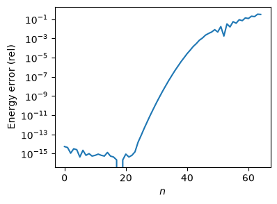
As a quick check, we consider the spectrum of a Harmonic oscillator with exact energies

\[\begin{gather*} E_n = \hbar \omega (n + \tfrac{1}{2}). \end{gather*}\]

If we want 20 states, then we must choose a basis where \(\hbar^2 K^2/2m > \hbar\omega (20.5)\) giving an estimate of \(K > 6.4/a_0\) where \(a_0 = \sqrt{\hbar/m\omega}\) is the oscillator length. We also need to make sure that the basis is large enough in position space. This state will have turning point \(R = \sqrt{2 E_{20}/m\omega^2} \approx 6.4a_0\) which means we need \(n \pi / K > R\). A bit of playing shows that \(Ka_0 = 10\) works well, which requires \(n > 6.4 K/\pi \approx 20\). Again, playing, we find that \(n = 30\) works well. Thus, we can get 20 states to machine precision with about 61 basis vectors.

def get_err_HO(Ka=10.0, N=30):
    hbar = m = w = 1
    a0 = np.sqrt(hbar/m/w)
    K = Ka/a0
    n = np.arange(-N, N+1)
    x = np.pi * n / Ka
    V = np.diag(m*(w*x)**2/2)
    n_, m_ = n[None, :], n[:, None]
    D2 = K**2 * np.ma.divide(2*(-1.0)**(n_ - m_)/np.pi**2, (m_-n_)**2).filled(1/3)
    K = hbar**2/2/m * D2
    H = K + V
    assert np.allclose(H, H.T)
    E = np.linalg.eigvalsh(H)
    exact = hbar*w * (np.arange(len(n)) + 0.5)
    err = abs(E/exact - 1)
    return err

fig, ax = plt.subplots(figsize=(4,3))
ax.semilogy(get_err_HO(Ka=10.0, N=32))
ax.set(xlabel="$n$", ylabel="Energy error (rel)");

From Orthogonal Polynomials

If the basis functions \(P_n(x)\) are orthogonal polynomials of degree \(n\), then we have an alternative and simpler path to a DVR basis. This section follows the ideas in [Schneider and Nygaard, 2004] but using a consistent notation with the previous section. Start with a basis and \(N\)-point Gaussian quadrature rule accurate for polynomials of degree \(2N-1\):

\[\begin{gather*} \braket{P_m|P_n} = \int w(x)\d{x}\; P_{n}^*(x)P_{m}(x) = \delta_{mn},\qquad \int w(x)\d{x}\; f(x) = \sum_{n} w_n f(x_n). \end{gather*}\]

Specifically, the quadrature rule is valid for \(f(x) = P_{n}^*(x)P_{m}(x)\) where \(n+m < 2N\).

The DVR basis is then

\[\begin{gather*} \ket{F_n} = \sum_{m}\ket{P_m}c_{mn}, \qquad F_n(x_m) = \sqrt{K_n}\delta_{mn}, \qquad \braket{F_{m}|F_{n}} = \delta_{mn}. \end{gather*}\]

For this to hold, the orthonormality and quadrature rules imply

\[\begin{gather*} c_{mn} = \braket{P_{m}|F_{n}} = \sum_{a} w_{a}P_{m}^*(x_a)F_{n}(x_a) %= \sum_{a} w_{a}P_{m}^*(x_a)\sqrt{K_{n}}\delta_{na} = w_{n}P_{m}^*(x_{n})\sqrt{K_{n}}\\ \braket{F_{m}|F_{n}} = \sum_{a} w_aF_m^*(x_a)F_n(x_a) = K_{n} w_{n}\delta_{mn}. \end{gather*}\]

Hence

\[\begin{gather*} K_{n} = \frac{1}{w_{n}}, \qquad c_{mn} = \sqrt{w_{n}}P_{m}^*(x_n),\qquad F_{n}(x) = \sqrt{w_{n}}\sum_{m}P_{m}^*(x_n)P_{m}(x). \end{gather*}\]

Since \(F_{n}(x)\) is a polynomial of degree \(N-1\) with \(N-1\) roots \(\{x_{m\neq n}\}\), we can express it as a Lagrange polynomial:

\[\begin{gather*} F_{n}(x) = \frac{1}{\sqrt{w_n}}\prod_{m}\frac{x-x_{m}}{x_{n}-x_{m}}. \end{gather*}\]

Some Technical Details

Let’s consider trying to construct a DVR basis from a general set of \(N\) orthogonal functions \(\ket{P_n}\) and abscissa \(x_n\):

\[\begin{gather*} \ket{F_i} = \sum_{n}\ket{P_n}U_{ni}, \qquad \braket{x_m|F_i} = \sqrt{K_m}\delta_{mi}, \qquad \braket{F_a|F_b} = \delta_{ab}. \end{gather*}\]

For these to be consistent we need

\[\begin{gather*} \sum_{n}P_{n}(x_m)U_{ni} = \sqrt{K_m}\delta_{mn}. \end{gather*}\]

In matrix notation, we need

\[\begin{gather*} [\mat{M}]_{mn} = P_{n}(x_m), \qquad [\mat{U}]_{ni} = U_{ni},\\ \mat{M}\mat{U} = \mat{D} = \diag(\sqrt{K}), \qquad \mat{U}^\dagger\mat{U} = \mat{1}. \end{gather*}\]

Thus, consistency requires that the matrix \(\mat{M}\) can be diagonalized by right-multiplying by a unitary matrix \(\mat{U}\).

This is true in finite-dimensional spaces, but might need some care in infinite dimensional spaces since there \(\mat{c}^\dagger\mat{c} = \mat{1}\) might not imply that \(\mat{c}\mat{c}^\dagger = \mat{1}\).

This requires that

\[\begin{gather*} \mat{M}\mat{U}\mat{U}^\dagger\mat{M}^\dagger = \mat{M}\mat{M}^\dagger = \abs{\mat{D}}^2 = \diag(K). \end{gather*}\]

This means that the abscissa must be chosen so that the rows of \(\mat{M}\). These are the vectors \(P_n(x)\) consisting of the basis functions evaluated at each colocation point \(x=x_{i}\).

It is not clear we can always do this: We have \(N\)-degrees of freedom – the locations of the abscissa \(x_{n}\) – but must satisfy \(N(N-1)/2\) conditions for the upper triangular portion of \(\mat{M}\mat{M}^{\dagger}\) to be zero.

For orthonormal polynomials, this orthogonality follows from the Christoffel–Darboux formula

\[\begin{gather*} \sum_{n=0}^{N-1} \frac{P_{n}(x)P_{n}(y)}{\braket{P_n|P_n}} = \sum_{n=0}^{N-1} \braket{x|P_n}\braket{P_n|y} = A_{N}\frac{P_{N}(x)P_{N-1}(y) - P_{N-1}(x)P_{N}(y)}{x-y} \end{gather*}\]

if we choose the abscissa to be the roots of \(P_{N}(x_n)=0\). Other functions satisfy a similar identity, including the Bessel functions [],

\[\begin{gather*} \sum_{k=1}^{\infty} 2(\nu+k)J_{\nu+k}(x)J_{\nu+k}(y) = \frac{xy}{x-y}\Bigl(J_{\nu+1}(x)J_{\nu}(y) - J_{\nu}(x)J_{\nu+1}(y)\Bigr)\\ 2(\nu+1)\sum_{k=1}^{\infty} 2(\nu+2k)J_{\nu+2k}(x)J_{\nu+2k}(y) = \frac{x^2y^2}{x^2-y^2}\Bigl(J_{\nu+2}(x)J_{\nu}(y) - J_{\nu}(x)J_{\nu+2}(y)\Bigr), \end{gather*}\]

and Airy functions

Basis Functions

We start with basis functions – typically some set of orthogonal polynomials \(P_n(x)\), but these can be more general, including Fourier bases (sines and cosines). Most convenient are functions orthogonal with respect to some integration weight \(w(x)\):

\[\begin{gather*} \braket{P_{m}|P_{n}} = \int \d{x}\; w(x) P_{m}^*(x) P_{n}(x) = \delta_{mn}. \end{gather*}\]

Bessel

The Bessel function basis is suitable for the radial coordinate in cylindrical and spherical geometries.

close relationship with Fourier series gives rise to many interesting properties of this basis.

\[\begin{gather*} P_{n}(x) = J_{\nu}(nx), \qquad P_{0}(x) = \frac{T_0(x)}{\sqrt{\pi}}, \qquad P_{n>0}(x) = \sqrt{\frac{2}{\pi}}T_{n}(x),\\ w(x) = \frac{1}{\sqrt{1-x^2}}, \qquad \braket{P_{m}|P_{n}} = \int_{-1}^{1} \d{x}\; \frac{P_{m}(x)P_{n}(x)}{\sqrt{1-x^2}} = \delta_{mn}. \end{gather*}\]

Fourier

The Fourier basis consists of plane waves, orthogonal on a periodic interval:

\[\begin{gather*} P_{n}(x) = e^{\I k_{n} x}, \qquad k_{n} = \frac{2\pi n}{L}, \qquad w(x) = \frac{1}{L}\\ \braket{k_{m}|k_{p}} = \frac{1}{L}\int_{0}^{L} \d{x}\; e^{-\I k_{m}x}e^{\I k_{n}x} = \delta_{mn}. \end{gather*}\]

Chebyshev

The Chebyshev basis is a transformed cosine basis to the interval \(x\in [-1, 1]\). The close relationship with Fourier series gives rise to many interesting properties of this basis.

\[\begin{gather*} T_{n}(x) = \cos(n\cos^{-1} x), \qquad P_{0}(x) = \frac{T_0(x)}{\sqrt{\pi}}, \qquad P_{n>0}(x) = \sqrt{\frac{2}{\pi}}T_{n}(x),\\ w(x) = \frac{1}{\sqrt{1-x^2}}, \qquad \braket{P_{m}|P_{n}} = \int_{-1}^{1} \d{x}\; \frac{P_{m}(x)P_{n}(x)}{\sqrt{1-x^2}} = \delta_{mn}. \end{gather*}\]

The idea is to express your functions in terms of this basis:

\[\begin{gather*} f(x) = \sum_{n} a_n P_n(x). \end{gather*}\]

Then the properties of the basis functions – such as their derivatives – can be used to calculate properties of \(f(x)\).

Do It! Use a Fourier Basis to do the first example in [Boyd, 1989].

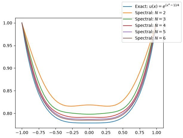
In §1.2, [Boyd, 1989] solves the following equation using a low-order polynomial expansion:

\[\begin{gather*} u_{,xx} - (x^6 + 3x^2)u = 0, \qquad u(-1) = u(1) = 1. \end{gather*}\]

Read the solution there, then repeat that analysis using a Fourier basis using everything you learn, including appropriately chosen collocation points, and considering the discussion about \(a_1 = 0\).

{solution}

As Boyd points out, the solutions must be even (prove this!), hence we need only consider a cosine series. The boundary conditions can be enforced with a series of the form

\[\begin{gather*} u(x) = 1 + \sum_{n=0}^{\infty} a_n\cos(k_n x), \qquad k_n = \bigl(n-\tfrac{1}{2}\bigr)\pi. \end{gather*}\]

Considering two terms \(a_0\) and \(a_1\), we choose the Gauss-Chebyshev collocation points: the roots of \(\phi_{1}(x) = \cos(k_1 x) = \cos(\pi x/2) = 0\):

\[\begin{gather*} k_0 = \frac{\pi}{2}, \qquad k_1 = \frac{3\pi}{2}, \\ x_{0} = \frac{1}{2}, \qquad x_{1} = 1. \end{gather*}\]

Plugging the solution into the equation gives us the residual function, which we set to zero at each of the collocation points

\[\begin{gather*} -(x_{i}^6 + 3x_{i}^2) + \sum_{n}\Bigl( -k_n^2 - (x_{i}^6 + 3x_{i}^2) \Bigr)a_n\cos(k_n x_{i}) = 0\\ -\left( \frac{\pi^2}{4} + \Bigl(\frac{1}{2^6} + \frac{3}{2^3}\Bigr) \right)a_0 -\left( \frac{\pi^2}{4} + \Bigl(\frac{1}{2^6} + \frac{3}{2^3}\Bigr) \right)(a_0\cos\tfrac{\pi = \Bigl(\frac{1}{2^6} + \frac{3}{2^3}\Bigr),\\ -\left( \frac{9\pi^2}{4} + \Bigl(1 + 3\Bigr) \right)a_1 = \Bigl(1+3\Bigr),\\ \begin{pmatrix} \frac{\pi^2}{4} + \frac{7}{8}\\ \end{pmatrix} \begin{pmatrix} a_0\\ a_1 \end{pmatrix} = \begin{pmatrix} \frac{7}{8}\\ 4 \end{pmatrix}N \end{gather*}\]

import sympy
def get_spectral_approx(N, show=False):
    an = sympy.symbols(f'a:{N}', real=True)
    kn = tuple(sympy.pi * (2*n + 1)/2 for n in sympy.S(np.arange(N)))
    xi = tuple((2*n+1)/(2*N+1) for n in sympy.S(np.arange(N)))
    print(xi)
    #xi = tuple(sympy.cos(sympy.pi * (N-n)/2/N) for n in sympy.S(np.arange(N)))
    x = sympy.symbols('x')
    u = 1 + sum(a_ * sympy.cos(k_ * x) for a_, k_ in zip(an, kn))
    Eqs = [(u.diff(x,x) - (x**6 + 3*x**2)*u).subs([(x, x_)]).evalf() for x_ in xi]
    sol = sympy.solve(Eqs, an)
    u_x = u.subs(sol)
    if show:
        display(sol)
        display(u.evalf())
    u_ = sympy.lambdify(x, u_x, "numpy")
    return u_

fig, ax = plt.subplots()
x = np.linspace(-1, 1)
u_exact = np.exp((x**4-1)/4)
ax.plot(x, u_exact, label="Exact: $u(x) = e^{(x^4-1)/4}$")
for N in [2, 3, 4, 5, 6]:
    u = get_spectral_approx(N=N)
    ax.plot(x, u(x), label=f"Spectral: ${N=}$")
fig.legend()

(1/5, 3/5)
(1/7, 3/7, 5/7)
(1/9, 1/3, 5/9, 7/9)
(1/11, 3/11, 5/11, 7/11, 9/11)
(1/13, 3/13, 5/13, 7/13, 9/13, 11/13)

<matplotlib.legend.Legend at 0x7bb3f8cc0980>

Numerical Example: Chebyshev Basis

We will explore these more in Spectral Methods: Chebyshev Basis, but for now, we give a couple of simplex examples using the Chebyshev polynomials \(T_{n}(x)\), which form a basis for functions on the interval \(x\in [-1, 1]\):

\[\begin{gather*} T_{n}(x) = \cos(n\cos^{-1}x). \end{gather*}\]

Example 1: Derivatives

We start by using the basis the approximate a function \(f(x)\) and then to compute its derivative. Let’s consider \(f(x) = e^{x}\): to determine the coefficients \(a_{n}\) we define a residual which we minimize. There are many ways of doing this – for example:

\[\begin{gather*} R(\vect{a}) = \int_{-1}^{1}\frac{\d{x}}{\sqrt{1-x^2}} \Bigl(f(x) - \sum_{n}a_n T_n(x)\Bigr)^2. \end{gather*}\]

To better work with this, we introduce the vectors \(\ket{f}\) (the function) an \(\ket{f_{\vect{a}}}\) (the approximation):

\[\begin{gather*} \braket{f|g} = \int_{-1}^{1}\frac{\d{x}}{\sqrt{1-x^2}} f^*(x) g(x),\\ \ket{f_{\vect{a}}} = \sum_{n}\ket{T_n}a_{n} = \ket{\vect{T}}\cdot\vect{a},\\ \braket{x|f} = f(x), \qquad \braket{x|t_{\vect{x}}} = \sum_{n}a_{n}\braket{x|T_{n}} = \sum_{n}a_nT_{n}(x). \end{gather*}\]

The residue, can then be expressed:

\[\begin{gather*} R(\vect{a}) = \braket{f|f} - 2\braket{f|f_{\vect{a}}} + \braket{f_{\vect{a}}|f_{\vect{a}}}. \end{gather*}\]

Approximate the ground state energy and wavefunction for a particle in a box with a Gaussian barrier:

\[\begin{gather*} V(x) = \begin{cases} V_0 e^{-x^2/2\sigma^2} & -1 < x < 1,\\ \infty & \text{otherwise}. \end{cases} \end{gather*}\]

DVR Bases

Slightly more generally, we can define the inner-product in terms of a Lebesque-Stieltjes integral with a measure \(\alpha(x)\), which is any non-decreasing function on the real numbers \(\alpha: \mathbb{R} \mapsto \mathbb{R}\):

\[\begin{gather*} \braket{P_m|P_n} = \int P_m^*(x)P_n(x) \d{\alpha(x)}. \end{gather*}\]

The relationship to the weight function \(w(x)\) is \(\d{\alpha(x)} = w(x)\d{x}\): i.e. \(w(x) = \alpha'(x)\). For example, the Lebesque-Stieltjes with \(\alpha(x) = \Theta(x)\) rigorously defines what we mean by a Dirac delta function weight \(w(x) = \delta(x)\).

To construct a DVR basis, one needs in addition to the basis, a quadrature rule. Thus, we need:

1. A set of \(N\) orthonormal basis functions \(P_{n}(x)\).

2. An \(N\)-point Gaussian quadrature rule exact for all linear and quadratic products of the basis functions.

As before, orthonormality is defined with respect to an inner product

\[\begin{gather*} \braket{P_m|P_n} = \int\d{x}\; w(x)P_m^*(x)P_n(x) = \delta_{mn}, \end{gather*}\]

and the \(N\)-point quadrature rule consists of \(N\) points \(x_i\) and weights \(w_i\) such that

\[\begin{gather*} \int \d{x}\; w(x)f(x) = \sum_{i} w_i f(x_i). \end{gather*}\]

For a DVR basis, we need this quadrature formula to be exact for:

1. The functions: \(P_n(x)\).

2. Products: \(P_m^*(x)P_n(x)\).

3. Products with an additional factor of \(x\): \(xP_m^*(x)P_n(x)\). (This is not strictly needed, but ensures that keeping the potential diagonal works reasonably well.)

This will be the case for the orthogonal polynomials, which is why we use the notation \(P_n(x)\), but also holds for the Fourier basis and some other sets with appropriately chosen quadrature rules.

From these ingredients, we construct a set of coordinate basis functions \(F_n(x)\) that are local in the sense that \(F_n(x_m)\) vanishes unless \(m=n\), and that are orthonormal with respect to the coordinate \(x\):

\[\begin{gather*} F_m(x) = \sum_{n} c_{mn}P_n(x), \qquad F_m(x_n) = f_m\delta_{mn}, \\ \braket{F_m|F_n} = \delta_{mn}, \qquad \braket{F_m|x|F_n} = x_m\delta_{mn}. \end{gather*}\]

Using the orthonormality and evaluating the integrals with the quadrature rule, these properties give the relationship:

\[\begin{gather*} c_{mn} = \int \d{x}\; w(x) P_{n}^*(x)F_{m}(x) = \sum_{i} w_i P_{n}^*(x_i)F_{m}(x_i) = w_m P_{n}^*(x_m)f_m,\\ \delta_{mn} = \int \d{x}\; w(x) F_m^*(x)F_n(x) = \sum_{i} w_i F_m^*(x_i)F_n(x_i) = w_m \abs{f_m}^2. \end{gather*}\]

Other Notations and the Cardinal Functions

To compare with the literature, note that [Schneider and Nygaard, 2004] uses the notation \(u_n(x) = \sqrt{w(x)}F_n(x)\) so that expectation values are simple

\[\begin{gather*} \braket{u_m|A(x)|u_n} = \int \d{x}\; u_m^*(x) A(x) u_n(x). \end{gather*}\]

This is convenient for numerical work.

In the notation of [Littlejohn et al., 2002], \(K_m = 1/w_m\). They use the following three functions, which differ only by normalization:

\[\begin{gather*} \Delta_n(x) = \sqrt{K_n}F_n(x) = K_n L_n(x),\\ \frac{\braket{\Delta_m|\Delta_n}}{K_m} = \braket{F_m|F_n} = K_m\braket{L_m|L_n} = \delta_{mn}\\ \frac{\Delta_{m}(x_n)}{K_{m}} = \frac{F_{m}(x_n)}{\sqrt{K_m}} = L_{m}(x_n) = \delta_{mn}. \end{gather*}\]

The functions \(L_{m}(x)\) here are denoted \(C_{m}(x)\) in [Boyd, 1989] and are called cardinal functions. These act like a Dirac delta function in the basis and can often be obtained by projection. For example, the cardinal functions for the Fourier basis can be constructed from (for even \(N\))

\[\begin{gather*} C_{m}(x) = \braket{x|C_{m}} = \frac{1}{N}\sum_{n}\braket{x|P_n}\braket{P_n|x_{m}} = \frac{1}{N}\sum_{n}P_{n}(x)P_{n}^*(x_m)\\ = \frac{1}{N}\sum_{n=-N/2}^{N/2-1}e^{\I k_{n}(x-x_m)} = \frac{1}{N}\sum_{n=-N/2}^{N/2-1}e^{2\pi \I n(x-x_m)/L}. \end{gather*}\]

This is geometric series:

\[\begin{gather*} S = \sum_{n=a}^{b} r^a = \frac{r^{b+1} - r^{a}}{1-r}, \qquad r = e^{2\pi \I (x-x_m)/L}, \qquad -a = b+1 = \frac{N}{2}. \end{gather*}\]

Thus,

\[\begin{gather*} C_{m}(x) = \frac{1}{N}\frac{e^{\pi N \I (x-x_m)/L} - e^{-\pi N \I (x-x_m)/L}} {1-e^{2\pi\I (x-x_m)/L}} = e^{-\pi\I (x-x_m)/L} \frac{\sin\frac{\pi N (x-x_m)}{L}}{N\sin\frac{\pi(x-x_m)}{L}}. \end{gather*}\]

The phase factor is somewhat inconsequential. (It results from the fact that, for even \(N\), there is a mismatch of positive and negative frequencies, so that the complex plane-wave \(P_{-N/2}(x)\) is unpaired. This issue can be removed, e.g., by shifting \(k_n \rightarrow k_n + \pi/L\), or by choosing \(N\) to be odd.) What remains are the cardinal functions for a periodic sine basis.

If we take the limit \(L \rightarrow \infty\) holding \(\d{x} = L/N\) fixed, then we recover the Whitaker cardinal functions (see the Whittaker-Shannon interpolation formula) for the real line:

\[\begin{gather*} \lim_{N, L \rightarrow \infty} C_{m}(x) = \frac{\sin\Big(k_c (x-x_m)\Bigr)}{k_c(x-x_m)} = \sinc\Big(k_c (x-x_m)\Bigr), \qquad k_c = \frac{\pi N}{L} = \frac{\pi}{\d{x}}. \end{gather*}\]

These can be solved, taking \(f_m\) to be real:

\[\begin{gather*} f_m = \frac{1}{\sqrt{w_m}}, \qquad c_{mn} = \sqrt{w_m}P_{n}^*(x_m), \qquad F_{m}(x) = \sqrt{w_m}\sum_{n}P_{n}^*(x_m)P_n(x). \end{gather*}\]

If the last quadrature condition is satisfied, then we have \(\braket{F_m|x|F_n} = x_m\delta_{mn}\), which gets to the essence of these basis: that the potential can be expressed as a diagonal matrix:

\[\begin{gather*} [\mat{V}]_{mn} = \braket{F_m|V(x)|F_n} = V(x_m)\delta_{mn}. \end{gather*}\]

To compute the kinetic energy, we must include factors of \(\sqrt{w(x)}\) in the basis functions:

\[\begin{gather*} u_n(x) = \sqrt{w(x)}F_{n}(x). \end{gather*}\]

Then, the kinetic energy can be evaluated using integration by parts and the quadrature rule. See below for details.

Orthogonal Polynomials

The integral \(\int \d{\alpha(x)}\) is a Lebesque-Stieltjes integral with measure \(\alpha(x)\), which should be a non-decreasing function on the reals. More commonly, we write \(\d{\alpha(x)} = w(x)\d{x}\) where \(w(x) = \alpha'(x)\) is called the weight function, but this is less general/more ambiguous. E.g. \(\alpha(x) = \Theta(x)\) rigorously defines what we mean by a Dirac delta function \(w(x) = \delta(x)\).

One way of constructing a DVR basis is from a set of \(N\) polynomials \(P_n(x)\) (i.e. of maximum degree \(N-1\)) that are orthonormal with respect to a measure \(\alpha(x)\):

\[\begin{gather*} \braket{P_m|P_n} = \int P_m(x)P_n(x) \d{\alpha(x)}. \end{gather*}\]

An \(N\)-point Gaussian quadrature rule is a set of \(N\) points \(x_i\) and weights \(w_i\) such that

\[\begin{gather*} \int P(x)\d{\alpha} = \sum w_i f(x_i) \end{gather*}\]

is exact for all polynomials of degree \(2N-1\) or less. To be used in constructing the DVR basis, the quadrature rule must be exact for polynomials of order \(2(N-1) + 1 = 2N-1\), thus, the Gaussian quadrature provides an acceptable set of \(N\) abscissa and weights for constructing the DVR basis using the formulae above.

Aliasing and Conservation Laws

This discussion remains true in 3D. In 1D there are infinitely many conserved quantities since the system is integrable. I expect there are pseudo-spectral formulations with as many conserved quantities as degrees of freedom.

In the continuum limit with constant external potential, the GPE conserves particle number, energy, and momentum:

\[\begin{align*} \DeclareMathOperator{\Im}{Im} N &= \int \abs{\psi}^2\d{x}, & E &= \int \left(\frac{\hbar^2\abs{\vect{\nabla}\psi}^2}{2m} + \frac{g\abs{\psi}^4}{2} \right)\d{x}, & \vect{ȷ} &= \Im \int (\psi^\dagger\hbar\vect{\nabla}\psi)\d{x}. \end{align*}\]

To see this, use the GPE

\[\begin{gather*} \I \hbar \dot{\psi} = \underbrace{\Biggl(\frac{-\hbar^2\nabla^2}{2m} + g\abs{\psi}^2\Biggr)} _{\op{H}_{\psi}}\psi. \end{gather*}\]

Consider the conservation of momentum:

\[\begin{gather*} \dot{\vect{ȷ}} = \Re \int \Biggl( \psi^\dagger\vect{\nabla}(\op{H}_{\psi}\psi) - (\op{H}_{\psi}\psi)^\dagger\vect{\nabla}\psi \Biggr) \d{x}. \end{gather*}\]

The contributions from the kinetic energies poses will cancel since derivatives commute, but the non-linear potential requires an application of the product rule:

\[\begin{gather*} \dot{\vect{ȷ}} = g\Re \int \Biggl( \psi^\dagger\vect{\nabla}(\abs{\psi}^2\psi) - \abs{\psi}^2 \psi^\dagger\vect{\nabla}\psi \Biggr) \d{x} = g\Re \int \Biggl( \psi^\dagger\psi\vect{\nabla}(\abs{\psi}^2) + \abs{\psi}^2\psi^\dagger\vect{\nabla}\psi - \abs{\psi}^2 \psi^\dagger\vect{\nabla}\psi \Biggr) \d{x},\\ = g\Re \int \Biggl(\abs{\psi}^2\vect{\nabla}(\abs{\psi}^2)\Biggr) \d{x},\ \end{gather*}\]

Nx = 64
Lx = 10.0
dx = Lx/Nx
k = 2*np.pi * np.fft.fftfreq(Nx, dx)
k_max = abs(k).max()
x = np.arange(Nx) * dx - Lx//2

Dk = 1j*k
Dk[Nx//2] = 0
D2k = -k**2

def P(f, kc):
    return np.fft.ifft(np.where(abs(k)<kc, np.fft.fft(f), 0))
    
def D(f):
    return np.fft.ifft(Dk*np.fft.fft(f))

def D2(f):
    return np.fft.ifft(D2k*np.fft.fft(f))

rng = np.random.default_rng(seed=2)
psi = rng.normal(size=2*Nx).view(complex)

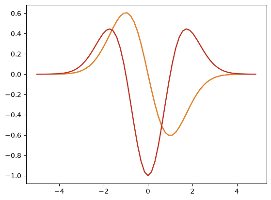
f = np.exp(-x**2/2)
df = -x*f
d2f = (x**2-1)*f

plt.plot(x, df)
plt.plot(x, D(f))
plt.plot(x, d2f)
plt.plot(x, D2(f))

/home/docs/checkouts/readthedocs.org/user_builds/gpe/conda/latest/lib/python3.14/site-packages/matplotlib/cbook.py:1719: ComplexWarning: Casting complex values to real discards the imaginary part
  return math.isfinite(val)
/home/docs/checkouts/readthedocs.org/user_builds/gpe/conda/latest/lib/python3.14/site-packages/matplotlib/cbook.py:1355: ComplexWarning: Casting complex values to real discards the imaginary part
  return np.asarray(x, float)

[<matplotlib.lines.Line2D at 0x7bb3f8b7c6e0>]

Consider

References

• [] has the best overview I have seen for the general formulation of DVR bases.