import mmf_setup

mmf_setup.nbinit()
%pylab inline --no-import-all

$\newcommand{\vect}[1]{\mathbf{#1}} \newcommand{\uvect}[1]{\hat{#1}} \newcommand{\abs}[1]{\lvert#1\rvert} \newcommand{\norm}[1]{\lVert#1\rVert} \newcommand{\I}{\mathrm{i}} \newcommand{\ket}[1]{\left|#1\right\rangle} \newcommand{\bra}[1]{\left\langle#1\right|} \newcommand{\braket}[1]{\langle#1\rangle} \newcommand{\Braket}[1]{\left\langle#1\right\rangle} \newcommand{\op}[1]{\mathbf{#1}} \newcommand{\mat}[1]{\mathbf{#1}} \newcommand{\d}{\mathrm{d}} \newcommand{\D}[1]{\mathcal{D}[#1]\;} \newcommand{\pdiff}[3][]{\frac{\partial^{#1} #2}{\partial {#3}^{#1}}} \newcommand{\diff}[3][]{\frac{\d^{#1} #2}{\d {#3}^{#1}}} \newcommand{\ddiff}[3][]{\frac{\delta^{#1} #2}{\delta {#3}^{#1}}} \newcommand{\floor}[1]{\left\lfloor#1\right\rfloor} \newcommand{\ceil}[1]{\left\lceil#1\right\rceil} % The following allows KaTeX to render these for significantly improved % performance on CoCalc. \newcommand{\DeclareMathOperator}[2]{\newcommand{#1}{#2}} \DeclareMathOperator{\Tr}{Tr} \DeclareMathOperator{\erf}{erf} \DeclareMathOperator{\erfi}{erfi} \DeclareMathOperator{\sech}{sech} \DeclareMathOperator{\sn}{sn} \DeclareMathOperator{\cn}{cn} \DeclareMathOperator{\dn}{dn} \DeclareMathOperator{\sgn}{sgn} \DeclareMathOperator{\order}{O} \DeclareMathOperator{\diag}{diag} % \newcommand{\mylabel}[1]{\label{#1}\tag{#1}} \newcommand{\degree}{\circ}$

This cell adds /home/docs/checkouts/readthedocs.org/user_builds/gpe/checkouts/latest/src to your path, and contains some definitions for equations and some CSS for styling the notebook. If things look a bit strange, please try the following:

• Choose "Trust Notebook" from the "File" menu.
• Re-execute this cell.
• Reload the notebook.

%pylab is deprecated, use %matplotlib inline and import the required libraries.
Populating the interactive namespace from numpy and matplotlib

Travelling Waves: Shooting

Here we consider shooting for solutions to the traveling wave problem. For more discussion see:

• Travelling Waves

GPE

We start with solutions to the GPE in 1D:

\[ \I\hbar \dot{\psi}(x, t) = -\frac{\hbar^2\psi''(x, t)}{2m} + g\abs{\psi(x, t)}^2\psi(x, t). \]

Implementing a full Galilean transformation, we have

\[\begin{split} \psi(x, t) = \sqrt{\rho_V(x_V)}e^{\I[\phi(x_V) - \mu t/\hbar]}e^{\I\bigl[mVx_V + \tfrac{m}{2}V^2t \bigr]/\hbar} = \psi_{V}(x_V)e^{\I\bigl[mVx_V + \bigl(\tfrac{m}{2}V^2 - \mu\bigr)t \bigr]/\hbar},\\ \mu\psi_V(x_V) = -\frac{\hbar^2\psi_V''(x_V)}{2m} + g\abs{\psi_V(x_V)}^2\psi_V(x_V),\\ \psi_V''(x_V) = \frac{2m}{\hbar^2}\left(g\abs{\psi_V(x_V)}^2-\mu\right)\psi_V(x_V). \end{split}\]

This is a complex-valued ODE which we can solve by shooing. Using the global phase invariance and translational invariance, we can assume that at \(x_V=0\), the wavefunction is real and has maximum density. With the parametrization \(\psi_V(x) = \sqrt{n(x)}e^{\I x k(x)}\) this means:

\[ n(x) = n_0 + \tfrac{1}{2}n''(0)x^2 + \order(x^3),\qquad k(x) = k_0 + \order(x^2). \]

(It might not be obvious that \(k'(0) = 0\), but expanding the GPE about \(x=0\) and collecting the imaginary parts of the \(x^2\) terms in the GPE requires this.)

\[\begin{split} \psi_V(0) = \sqrt{n_0}, \qquad \psi_V'(0) = \I k_0\sqrt{n_0},\quad \psi_V''(0) = \frac{n_0'' - 2n_0k_0^2}{2\sqrt{n_0}},\\ \frac{\hbar^2 n_0''}{4mn_0} = \overbrace{\frac{\hbar^2 k_0^2}{2m}}^{E_0} + gn_0 - \mu \leq 0. \end{split}\]

Thus, we have a continuous family of solutions with \(0 < n_0 < (\mu-E_0)/g\). As independent parameters we may take \(\hbar\), \(m\), \(g\), specifying units, and \(0<n_0\), \(0<f=gn_0/(\mu-E_0)<1\), and \(k_0\) specifying the solution.

Numerical Example

Here we numerically solve this equation using the scipy IVP solver, then compare this with our exact solution as implemented in the gpe.exact_solutions.TravellingWave class.

from scipy.integrate import solve_ivp


class ODE:
    hbar = 1.0
    g = 1.0
    m = 1.0
    periods = 3

    n0 = 1.0
    fraction = 0.9
    k0 = 0.0

    @property
    def mu(self):
        return self.g * self.n0 / self.fraction + self.E0

    @property
    def E0(self):
        return (self.hbar * self.k0) ** 2 / 2 / self.m

    @property
    def y0(self):
        """Return the initial state"""
        psi0 = np.sqrt(self.n0)
        dpsi0 = 1j * self.k0 * psi0
        return (psi0, dpsi0)

    def f(self, x, y):
        psi, dpsi = y
        ddpsi = 2 * self.m * (self.g * np.abs(psi) ** 2 - self.mu) * psi / self.hbar**2
        return (dpsi, ddpsi)

    def event(self, x, y):
        """Termination when dpsi=0 again"""
        if x <= 0:
            return -1
        psi, dpsi = y
        return dpsi.real

    event.terminal = True
    event.direction = -1

    def solve(self, max_step=0.1):
        x_max = 10.0
        ivp = solve_ivp(
            self.f,
            (0, x_max),
            self.y0,
            max_step=max_step,
            # events=[self.event],
        )
        return ivp


ode = ODE()
ode.k0 = 0.3
ode.fraction = 0.9
ode.n0 = 1.0
ode.f(0, ode.y0)

(0.3j, np.float64(-0.3122222222222222))

ivp = ode.solve()
print(ivp.message)
x, psi = ivp.t, ivp.y[0]
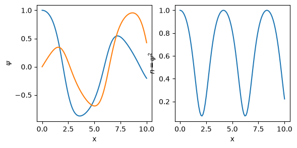
plt.figure(figsize=(10, 3))
ax1 = plt.subplot(131)
ax1.plot(x, psi.real)
ax1.plot(x, psi.imag)
ax1.set(xlabel="x", ylabel=r"$\psi$")
ax2 = plt.subplot(132)
ax2.plot(x, abs(psi) ** 2)
ax2.set(xlabel="x", ylabel=r"$n=\psi^2$")
# L = ivp.t_events[0]

The solver successfully reached the end of the integration interval.

[Text(0.5, 0, 'x'), Text(0, 0.5, '$n=\\psi^2$')]