Spectral Methods: Chebyshev Basis#
After the Fourier basis, then next most-useful basis is based on the Chebyshev polynomials, which can be expressed as
A function expressed in this basis will thus have the form
Thus, expressing a function \(f(x)\) for \(x\in [-1, 1]\) in this basis is equivalent to considering a periodic function \(F(\theta)\) with period \(2\pi\) on the interval \(\theta \in [0, \pi]\). These two representations are codified by the relationship:
The relationship between Chebyshev and Fourier bases
If the Chebyshev basis is just a Fourier basis on \(\theta\), where has the periodicity gone? The answer is that the periodic copies get mapped back into the interval \(x\in [-1,1]\): the choice of \(\theta \in [0, \pi]\) is because the mapping \(\cos \theta\) is single-values / invertable on this interval.
This transformation implies that
Hence, if \(f(x)\) is not singular, then \(F'(\theta) = 0\) at the boundaries of the interval \([0, \pi]\) where \(\sin \theta = 0\). Note however, that this does not imply any properties about the derivative \(f'(x)\) at the boundaries.
The Chebyshev polynomials are orthogonal with respect to the weight \(W(x) = 1/\sqrt{1-x^2} = 1/\sin\theta\):
Integration and Differentiation#
Having a spectral representation affords us analytic integration and differentiation formulae
Thus: if a function is exactly representable in the basis, then the derivative is exact, and the integral is almost exact except for the highest component.
We can use these as follows:
Each of these contains a discrete sine or cosine series that can be computed using the DCT and/or DST. For integration, it might be simpler just to shift the two series using the explicit formula, but this needs testing.
Some Details
To see this, note
after canceling the wrong term. To check the previous formula, note
These can be manipulated to derive expressions in the basis, but it is easier to work algebraically using recurrence relationships. To get an idea about how these work, first introduce the complementary Chebyshev polynomials of the second kind
These satisfy the following recurrence relations:
The first few of these are
To convert from one to the other:
functions
d2Tn_dx2 = dTn_dx.diff(th)/x.diff(th)
d2m = d2Tn_dx2.limit(th, sympy.pi).factor().simplify()
d2p = d2Tn_dx2.limit(th, 0).factor().simplify()
display(Latex(f"$T''_n(-1) = {sympy.latex(d2m)}$"))
display(Latex(f"$T''_n(+1) = {sympy.latex(d2p)}$"))
Pseudo-Spectral Chebyshev Basis#
The pseudo-spectral approach pairs a spectral basis \(\phi_{m}(x)\) with an appropriate set of abscissa \(x_{i}\). To be effective, one should be able to associate the grid with quadrature weights \(w_i\) such that
is exact for polynomials \(f(x)\) of degree \(N\) or less (with \(N\) abscissa).
There are two sets of quadrature points and weights based on the Chebyshev polynomials. Both are exact for polynomials of degree up to and including \(x^{2N-1}\) (i.e., with \(2N\) coefficients):
We also include here the Cardinal Functions (DVR) \(C_j(x)\) which are zero at all abscissa exact one
Chebyshev-Gauss (Interior Points / Roots)#
The \(N\) abscissa are the roots of \(T_{N}(x)\), which lie in the interior:
The \(N\) weights and \(N\) abscissa are free, allowing us to fit these \(2N\) independent parameters. The relevant DCTs and DSTs are:
Chebyshev-Gauss-Lobatto (Extrema + Endpoints)#
The \(N+1\) abscissa are the extrema of \(T_{N}(x)\) plus the endpoints:
Since we fix the endpoints, we have \(N+1\) weights and \(N-1\) free abscissa, giving \(2N\) free parameters. The relevant DCTs and DSTs are:
These are implemented in the gpe.chebyshev.Chebyshev with the slight
modification that the order of the points is changed so that the abscissa increase
rather than decrease.
Refinement#
Refining in the Chebyshev basis is trivial: to start resolving more features, simply add higher-order coefficients, setting them to zero.
Chebyshev Quadrature (Interior Points)
The roots of \(T_{N}(x_j) = 0\) are trivial:
The weights are thus
Numerical Check
Here we check the accuracy of these quadrature schemes using
(I found this from https://oeis.org/A001700.)
import sympy
th = sympy.var('theta')
[sympy.integrate(sympy.cos(th)**(2*n), (th, 0, sympy.pi))
                 * 2**(2*n-1) / sympy.pi
 for n in range(1, 12)]
import sympy
th = sympy.var('theta')
[sympy.integrate(sympy.cos(th)**(2*n), (th, 0, sympy.pi))
                 * 2**(2*n-1) / sympy.pi
 for n in range(1, 12)]
[1, 3, 10, 35, 126, 462, 1716, 6435, 24310, 92378, 352716]
# Chebyshev Quadrature
from functools import partial
import scipy.integrate
import scipy as sp

def get_xw1(N):
    """Return the N Chevbyshev absicssa and weights (interior points)."""
    j = np.arange(N)
    th = np.pi * (2*j + 1)/2/N
    x = np.cos(th)
    w = np.pi / N
    return x, w

def get_xw2(N):
    """Return the N+1 Chevbyshev-Lobatto absicssa and weights (extrema+endpoints)."""
    j = np.arange(N+1)
    th = np.pi * j / N
    x = np.cos(th)
    w = np.pi / N + 0*x
    w[0] /= 2
    w[-1] /= 2
    return x, w

# Three ways to check
# Sympy: This uses hypergeometric functions
import sympy
x = sympy.var('x')
n = sympy.var('n', integer=True, positive=True)
I_sympy = sympy.lambdify([n], sympy.integrate(x**n/sympy.sqrt(1-x**2), (x, -1, 1)), 'mpmath')

# Exact formula
def I_exact(n):
    if n == 0:
        return np.pi
    elif n %2  == 1:
        return 0
    elif n % 2 == 0:
        return np.pi * sp.special.binom(n - 1, n//2) / 2**(n-1)

# Adaptive quadrature
def W(x):
    return 1/np.sqrt(1-x**2)

def integrand(x, n):
    return x**n * W(x)

def I_quad(n):
    res, err = sp.integrate.quad(
        partial(integrand, n=n), -1, 1,
        epsabs=1e-11, epsrel=1e-12)
    return res, err
for N in range(1, 10):
ns = np.arange(2*N+1)
cheb1 = []
cheb2 = []
for n in ns:
x, w = get_xw1(N)
cheb1.append((w*x**n).sum())
x, w = get_xw2(N)
cheb2.append((w*x**n).sum())
exact = np.array([I_exact(n) for n in ns])
quad = [I_quad(n) for n in ns]
sym = [I_sympy(n) for n in ns]
assert np.allclose(exact[:-1], cheb1[:-1])
assert np.allclose(exact[:-1], cheb2[:-1])
assert not np.allclose(exact[-1], cheb1[1])
assert not np.allclose(exact[-1], cheb2[1])
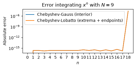
fig, ax = plt.subplots(figsize=(5, 2))
ax.semilogy(ns, abs(exact - cheb1), label="Chebyshev-Gauss (interior)")
ax.semilogy(ns, abs(exact - cheb1), label="Chebyshev-Lobatto (extrema + endpoints)")
ax.set(xlabel="$n$", xticks=ns,
ylabel="Absolute error",
title=f"Error integrating $x^n$ with ${N=}$")
ax.legend();
Derivatives and Integration#


Discrete Cosine/Sine Transforms (DCT/DST)
As with the FFT, one can use the DCT and DST to compute derivatives. There are
a variety of options differing in how the interval \(\theta \in [0, \pi]\) is extended to
a periodic function over \([0, 2\pi)\). DCT-I is periodic about the endpoints, and
hence suitable for the Gauss-Lobatto abscissa which have; DCT-2 is periodic about
the points outside of the see Periodic Extensions of the DCT. Here we discuss the appropriate formula
for the DCT (see scipy.fft.dct()).
The strategy is:
Use the DCT to change bases, finding the coefficients \(a_{k}\) such that
\[\begin{gather*} f_{j} = f(x_{j}) = \sum_{k}a_{k} T_{k}(x_{j}) = \sum_{k}a_{k} \cos (k \cos^{-1} x_{j}) = \sum_{k}a_{k} \cos (k \theta_{j}). \end{gather*}\]Compute the derivative:
\[\begin{align*} f'(x_{j}) &= \sum_{k}a_{k} T_{k}'(x_{j}) = \sum_{k}a_{k} (-k)\sin(k \theta_{j})\theta'_{j},\\ &= \sum_{k}a_{k} k\frac{\sin(k \theta_{j})}{\sin \theta_{j}},\\ f''(x_{j}) &= \sum_{k}a_{k} T_{k}''(x_{j}) = \sum_{k}a_{k} (-k)\sin(k \theta_{j})\theta'_{j},\\ &= \sum_{k}a_{k}\left( -k^2\frac{\cos(k \theta_{j})}{\sin^2 \theta_{j}} + k\frac{\sin(k \theta_{j})\cos \theta_j}{\sin^3\theta_{j}} \right). \end{align*}\]Use the DST and DCT to invert the transformation:
\[\begin{gather*} f_{j} = f(x_j) = \sum_{k}b_{k}\sin(k \theta_{j}) \end{gather*}\]
To do this in the code, we must choose the appropriate version of the DCT and DST, which differ in terms of the precise abscissa \(\theta_{j}\) used, offsets in the indices, and factors for the coefficients. We first summarize the relevant transformations.
DCT-I:
\[\begin{align*} \theta_{k} &= \left.\frac{k\pi}{N}\right|_{k=0}^{N},\\ [f_0, f_1, \cdots, f_{N}] & \mathrel{\substack{\text{iDCT-I}\\\rightleftharpoons\\\text{DCT-I}}} [a_0, \tfrac{1}{2}a_{1}, \cdots, \tfrac{1}{2}a_{N-1}, a_{N}]. \end{align*}\]DCT-II and DCT-III:
\[\begin{align*} \theta_{k} &= \left.\frac{(k+\tfrac{1}{2})\pi}{N}\right|_{k=0}^{N-1},\\ [f_0, f_1, \cdots, f_{N-1}] & \mathrel{\substack{\text{DCT-III = iDCT-II}\\\rightleftharpoons\\\text{DCT-II == iDCT-III}}} [\tfrac{1}{2}a_{0}, \cdots, \tfrac{1}{2}a_{N-1}]. \end{align*}\]DST-I:
\[\begin{align*} \theta_{k} &= \left.\frac{k\pi}{N+1}\right|_{k=1}^{N},\\ [f_1, f_2, \cdots, f_{N}] & \mathrel{\substack{\text{DST-I}\\\rightleftharpoons\\\text{iDST-I}}} [\tfrac{1}{2}a_{1}, \cdots, \tfrac{1}{2}a_{N}]. \end{align*}\]DST-III:
\[\begin{align*} \theta_{k} &= \left.\frac{k\pi}{N+1}\right|_{k=1}^{N},\\ [f_1, f_2, \cdots, f_{N}] & \mathrel{\substack{\text{DST-I}\\\rightleftharpoons\\\text{iDST-I}}} [\tfrac{1}{2}a_{1}, \cdots, \tfrac{1}{2}a_{N}]. \end{align*}\]
Type I:
From scipy.fft.dct(), changing only \(N \rightarrow N+1\), \(y_{k} \rightarrow
f_{k}\), and \(x_{n} \rightarrow \tilde{f}_{n}\) for notational convenience:
This matches the Gauss-Lobatto abscissa as shown with
The DCT-I as written thus effects the inverse transformation \(a_{n} \rightarrow f_{k}\), and the inverse effects the forward transform from \(f_{k} \rightarrow a_{n}\) with appropriate scaling by factors of 2.
Similarly, the derivatives can be computed using the DST-I. Here is what we need to compute derivatives with respect to \(\theta\), then we use the chain rule to compute \(f'(x)\):
I.e., each coefficient \(\tilde{f}_{n}\) is simply multiplied by \(-n\), and now we have a sine series. To convert this back to position space, we use the DST-I, which computes
Notice that we need to shift the coefficients. Finally, we need to use the chain rule to compute the derivative:
This is fine everywhere except at the endpoints where we must use L’Hôpital’s rule to obtain
The second derivative has the following properties. Let \(a_n = 2\tilde{f}_{n}\) except \(a_{N} = \tilde{f}_{N}\). Then
Type III
The DCT-II as written thus effects the inverse transformation \(a_{n} \rightarrow f_{k}\), and the inverse transform (the DCT-II) effects the forward transform from \(f_{k} \rightarrow a_{n}\) with appropriate scaling by factors of 2.
To compute derivatives, we note that
These can be computed using the DST-III with coefficients \(-\tilde{f}_{n}k_{n}\) shifted by one.
Similarly, the derivatives can be computed using the DST-II:
Similarly, the derivatives can be computed using the DST-III:
Similarly, the derivatives can be computed using the DST-IV:
Here we demonstrate these formula:
import scipy.fft
sp = scipy
# Gauss quadrature at roots (interior points)
N = 12
n1 = k1 = np.arange(N)
th1 = np.pi * (2*n1 + 1) / 2 / N
x1 = np.cos(th1)
def get_a1(f):
"""Return the expansion coefficients."""
ft = sp.fft.dct(f, type=2, norm='forward')
a = 2*ft
a[0] = ft[0]
return a
def get_f1(a):
"""Return the function in position space."""
ft = a/2
ft[0] = a[0]
return sp.fft.idct(ft, type=2, norm='forward')
def diff_1(f, d=1, th=th1, k=k1):
ft = sp.fft.dct(f, type=2, norm='forward')
s = np.sin(th)
# Shift the coefficients and pad with zero.
df_dth = sp.fft.dst(np.concatenate([-(ft*k)[1:], [0]]), type=3)
if d == 1:
df_dx = -df_dth / s
return df_dx
elif d >= 2:
d2f_dth2 = sp.fft.idct(-ft*k**2, type=2, norm='forward')
d2f_dx2 = (d2f_dth2 - df_dth / np.tan(th)) / s**2
if d == 2:
return d2f_dx2
return diff(d2f_dx2, d=d-2)
n2 = k2 = np.arange(N+1)
th2 = np.pi * n2 / N
x2 = np.cos(th2)
def get_a2(f):
"""Return the expansion coefficients."""
ft = sp.fft.idct(f, type=1, norm='backward')
a = 2*ft
a[0], a[-1] = ft[0], ft[-1]
return a
def get_f2(a):
"""Return the function in position space."""
ft = a/2
ft[0], ft[-1] = a[0], a[-1]
return sp.fft.dct(ft, type=1, norm='backward')
def diff_2(f, d=1, th=th2, k=k2):
ft = sp.fft.idct(f, type=1, norm='backward')
s = np.sin(th)
# Shift the coefficients and pad with zero.
df_dth = sp.fft.dst(np.concatenate([-(ft*k)[1:], [0]]), type=1)
if d == 1:
df_dx = -df_dth / s
return df_dx
elif d >= 2:
d2f_dth2 = sp.fft.dct(-ft*k**2, type=1, norm='backward')
d2f_dx2 = (d2f_dth2 - df_dth / np.tan(th)) / s**2
if d == 2:
return d2f_dx2
return diff(d2f_dx2, d=d-2)
def T(x, n):
return np.cos(n*np.acos(x))
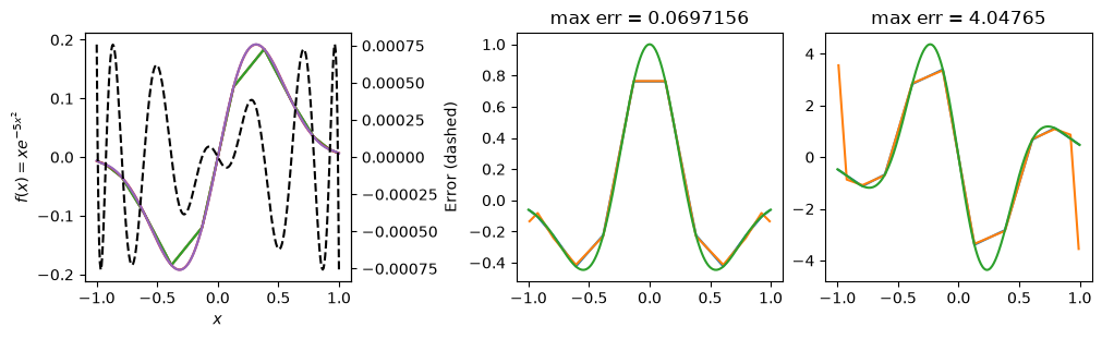
# Test
x_ = np.linspace(-1, 1, 300)
for (x, n, get_a, get_f, diff) in [
(x1, n1, get_a1, get_f1, diff_1),
(x2, n2, get_a2, get_f2, diff_2)]:
f = x * np.exp(-5*x**2)
df = (1 - 10*x**2)*np.exp(-5*x**2)
ddf = 10*x*(-3 + 10*x**2)*np.exp(-5*x**2)
f_ = x_ * np.exp(-5*x_**2)
df_ = (1 - 10*x_**2)*np.exp(-5*x_**2)
ddf_ = 10*x_*(-3 + 10*x_**2)*np.exp(-5*x_**2)
a = get_a(f)
f1 = get_f(a)
df1 = diff(f, d=1)
ddf1 = diff(f, d=2)
f2 = T(x[:, None], n[None, :]) @ a
f1_ = T(x_[:, None], n[None, :]) @ a
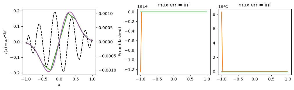
fig, axs = plt.subplots(1, 3, figsize=(10, 3), constrained_layout=True)
ax = axs[0]
ax.plot(x, f)
ax.plot(x, f1)
ax.plot(x, f2)
ax.plot(x_, f_)
ax.plot(x_, f1_)
ax1 = ax.twinx()
ax1.plot(x_, f1_ - f_, '--k')
ax.set(xlabel="$x$", ylabel="$f(x) = xe^{-5x^2}$")
ax1.set(ylabel="Error (dashed)");
axs[1].plot(x, df)
axs[1].plot(x, df1)
axs[1].plot(x_, df_)
axs[1].set(title=f"max err = {abs(df-df1).max():g}")
axs[2].plot(x, ddf)
axs[2].plot(x, ddf1)
axs[2].plot(x_, ddf_)
axs[2].set(title=f"max err = {abs(ddf-ddf1).max():g}");
/tmp/ipykernel_4825/3423782851.py:64: RuntimeWarning: divide by zero encountered in divide
  df_dx = -df_dth / s
/tmp/ipykernel_4825/3423782851.py:68: RuntimeWarning: divide by zero encountered in divide
  d2f_dx2 = (d2f_dth2 - df_dth / np.tan(th)) / s**2
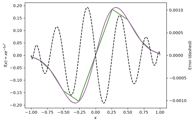
import scipy.fft
sp = scipy

# Gauss-Lobatto quadrature at extrema and endpoints

N = 12
n = k = np.arange(N+1)
th = np.pi * n / N
x = np.cos(th)

def get_a2(f):
    """Return the expansion coefficients."""
    ft = sp.fft.idct(f, type=1, norm='backward')
    a = 2*ft
    a[0], a[-1] = ft[0], ft[-1]
    return a

def get_f2(a):
    """Return the function in position space."""
    ft = a/2
    ft[0], ft[-1] = a[0], a[-1]
    return sp.fft.dct(ft, type=1, norm='backward')

def T(x, n):
    return np.cos(n*np.acos(x))

# Test
x_ = np.linspace(-1, 1, 300)
f = x * np.exp(-5*x**2)
f_ = x_ * np.exp(-5*x_**2)
a = get_a2(f)
f1 = get_f2(a)
f2 = T(x[:, None], n[None, :]) @ a
f1_ = T(x_[:, None], n[None, :]) @ a

fig, ax = plt.subplots()
ax.plot(x, f)
ax.plot(x, f1)
ax.plot(x, f2)
ax.plot(x_, f_)
ax.plot(x_, f1_)
ax1 = ax.twinx()
ax1.plot(x_, f1_ - f_, '--k')
ax.set(xlabel="$x$", ylabel="$f(x) = xe^{-5x^2}$")
ax1.set(ylabel="Error (dashed)");
Here is a simple implementation:
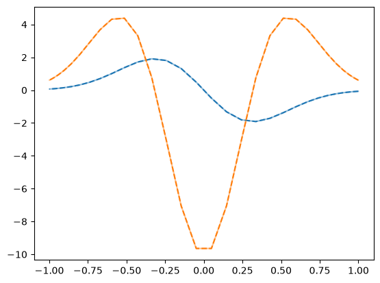
import scipy.fft
sp = scipy

Nx = 32
n = m = np.arange(Nx)
th = np.pi * (2*m + 1)/2/Nx
k = n
x = np.cos(th)

def diff(f, d=1, k=k, th=th):
    ft = sp.fft.dct(f, type=2, norm='forward')
    s = np.sin(th)

    # Shift the coefficients and pad with zero.
    df_dth = sp.fft.dst(np.concatenate([-(ft*k)[1:], [0]]), type=3)
    if d == 1:
        df_dx = -df_dth / s
        return df_dx
    elif d == 2:
        d2f_dth2 = sp.fft.idct(-ft*k**2, type=2, norm='forward')
        d2f_dx2 = (d2f_dth2 - df_dth / np.tan(th)) / s**2
        return d2f_dx2
    return diff(df_dx, d=d-1)

f = np.exp(-5*x**2)
df = -10*x*f
ddf = (100 * x**2 - 10) * f

plt.plot(x, df, '-C0', alpha=0.5)
plt.plot(x, diff(f), '--C0')
plt.plot(x, ddf, '-C1', alpha=0.5)
plt.plot(x, diff(f, d=2), '--C1');
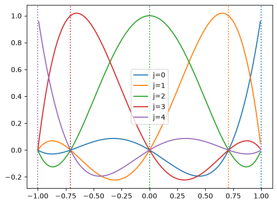
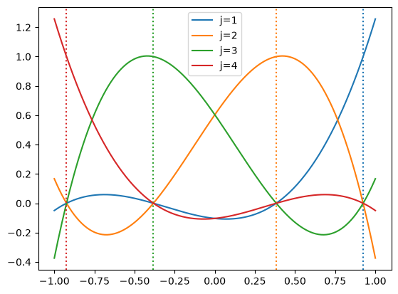
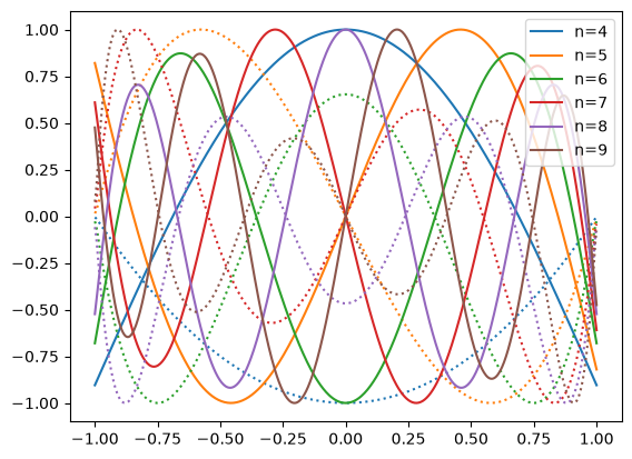
Cardinal Functions (DVR)#
The cardinal functions \(C_j(x)\) are rearrangements of the basis functions such that
One can think of these as the delta-functions for the basis. To expand a function in the basis using these, one simply needs to evaluate the function at the abscissa:
Two sets of cardinal functions are given for the Chebyshev basis in [Boyd, 1989]. To evaluate these, we must be able to accurately compute
Gauss-Lobatto Grid (Extrema)#
Roots Grid (Interior Points)#
def T(x, n, d=0):
    th = np.arccos(x)
    if d == 0:
        return np.cos(n*th)
    elif d == 1:
        return n*np.sin(n*th)/np.sin(th)

class Base:
    def __init__(self, **kw):
        for key in kw:
            if not hasattr(self, key):
                raise ValueError(f"Unknown {key=}")
            setattr(self, key, kw[key])
        self.init()

    def init(self):
        pass

class Basis1(Base):
    """Gauss-Lobatto Grid of extrema and endpoints."""
    N = 32
    def init(self):
        super().init()

    def get_x(self, j):
        return np.cos(np.pi * j / self.N)

    def get_C(self, x, j):
        N = self.N
        xj = self.get_x(j=j)
        C = (-1)**(j+1) * (1-x**2) / (x-xj) * T(x, N, d=1) / N**2
        if j == N or j == 0:
            C /= 2
        return C

b = Basis1(N=4)
x = np.linspace(-1, 1, 256)
fig, ax = plt.subplots()
for j in range(0, b.N+1):
    l, = ax.plot(x, b.get_C(x, j=j), label=f"{j=}")
    ax.axvline([b.get_x(j=j)], c=l.get_c(), ls=":")
ax.legend();
/tmp/ipykernel_4825/3661239913.py:31: RuntimeWarning: invalid value encountered in divide
  C = (-1)**(j+1) * (1-x**2) / (x-xj) * T(x, N, d=1) / N**2
/tmp/ipykernel_4825/3661239913.py:6: RuntimeWarning: invalid value encountered in divide
  return n*np.sin(n*th)/np.sin(th)
_EPS = np.finfo(float).eps

class Basis2(Base):
    """Interior points of Roots.

    Formulae from Appendix F of {cite}`Boyd:2001`.
    """
    N = 32

    def init(self):
        super().init()
        self.i = 1+np.arange(self.N)
        self.x = self.get_x(self.i)

    def get_x(self, j):
        return np.cos(np.pi * (2*j-1) / 2 / self.N)

    def get_C(self, x, j, d=0):
        N = self.N
        xj = self.get_x(j=j)
        t = np.arccos(x)
        tj = np.arccos(xj)
        return np.cos(N*t) * np.sin(tj) / N / np.sin(N*tj) / (np.cos(t) - np.cos(tj))

    def get_D1(self):
        """Return the derivative matrix."""
        i = self.i
        xi = self.x
        i, j = i[:, None], i[None, :]
        xi, xj = xi[:, None], xi[None, :]
        D1 = (-1)*(i+j)*np.sqrt((1-xj**2)/(1-xi**2))/(xi-xj+_EPS)
        D1 -= np.diag(np.diag(D1))
        xj = np.ravel(xj)
        D1 += np.diag(0.5*xj/(1-xj**2))
        return D1

    def get_D2(self):
        """Return the second derivative matrix."""
        N = self.N
        i = self.i
        xi = self.x
        i, j = i[:, None], i[None, :]
        xi, xj = xi[:, None], xi[None, :]
        D2 = self.get_D1() * (xi/(1-xi**2) - 2 / (xi-xj+_EPS))
        D2 -= np.diag(np.diag(D2))
        xj = np.ravel(xj)
        D2 += np.diag(xj**2/(1-xj**2)**2 - (N**2-1)/3/(1-xj**2))
        return D2

b = Basis2(N=4)
x = np.linspace(-1, 1, 256)
fig, ax = plt.subplots()
for j in range(1, b.N+1):
    l, = ax.plot(x, b.get_C(x, j=j), label=f"{j=}")
    ax.axvline([b.get_x(j=j)], c=l.get_c(), ls=":")
ax.legend();
A Chebyshev Basis with \(f''(\pm 1)=0\).
One solution is linearly combine states to ensure this boundary condition. Note that
Therefore:
Thus, \(T_0\) and \(T_1\) already have the correct boundaries. \(T_2\) and \(T_3\) don’t, so must be excluded, but can then be used to correct the basis functions. Here is a simple approach:
Unfortunately, these functions become highly degenerate because the corrections dominate for large \(n\). Instead, we can do the following:
Thus, given
This gives us the following recurrence
Nx = 32
n = m = np.arange(Nx)
th = np.pi * (2*m + 1) / 2/ Nx
k = n
x = np.cos(th)

f = np.sin(np.pi * x**2)
a = get_a1(f)
b = a.copy()
for n in range(Nx-3, 3, -1):
    b[n] = -a[n] + b[n+2]*(n+2)**2*(n+3)/n**2/(n-1)
b[2] = b[3] = 0
x = np.linspace(-1, 1, 500)
def T(x, n):
    return np.cos(n*np.acos(x))

def phi1(x, n):
    fact = n**2*(n**2 - 1)

    if n % 2 == 0:
        phi = T(x, n) - fact*T(x, 2)/12
    else:
        phi = T(x, n) - fact*T(x, 3)/72
    return phi / phi.max()

def phi2(x, n):
    fact = n**2*(n**2 - 1)/(n-2)**2/((n-2)**2 - 1)
    phi = T(x, n) - fact*T(x, n-2)
    return phi / abs(phi).max()

def d2(f):
    for n in range(2):
        f = np.gradient(f, x, edge_order=2)
    return f

for n in range(4, 10):
    l, = plt.plot(x, phi2(x, n), label=f"{n=}")
    d2_phi = d2(phi2(x, n))
    plt.plot(x, d2_phi/abs(d2_phi).max(), ':', c=l.get_c())
plt.legend();
The first spectral basis we will consider is provided by the Chebyshev polynomials of the first kind \(\{T_n(x)\}\) which are orthogonal on the interval \(x\in [-1, 1]\) with weighting function \(W(x) = 1/\sqrt{1-x^2}\):
The Chebyshev polynomials of the second kind \(U_{n}(x)\) are useful for computing derivatives:
If we express
from scipy.integrate import quad

def T(x, n):
    return np.cos(n*np.acos(x))

quad(lambda x: T(x,2)*T(x,2)/np.sqrt(1-x**2), -1, 1)
(1.5707963267948821, 1.75867045371092e-08)