Viscosity Notes 1#
These are some supporting notes for the document Effective Viscosity.
Numerical Potentials#
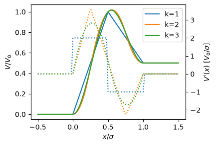
In Flow Past a Barrier, we want some potentials that have a barrier height \(V_0\), a width \(\sigma\), and a drop \(\delta\). This is easy to do with a splines:
from scipy.interpolate import InterpolatedUnivariateSpline

def V_linear(x, V0=0.5, sigma=2.0, dV=0.2, d=0, k=1):
    """Return the dth derivative of a linear potential barrier.

    Arguments
    ---------
    x : array-like
        Abscissa on which to compute the potential.
    V0 : float
        Height of barrier.
    sigma : float
        Width of barrier.
    dV : float
        Potential difference from right to left of the barrier.
    d : [0, 1]
        Derivative order.
    k : int
        Order of spline.
    """
    xp, fp = [0, sigma / 2, sigma], [0, V0, dV]
    if k > 1:
        xp = sigma * np.linspace(0, 1, 7)
        fp = [0] * 3 + [V0] + [dV] * 3
        xp = sigma * np.array([0, 0.001, 0.5, 0.999, 1])
        fp = [0] * 2 + [V0] + [dV] * 2
    V = InterpolatedUnivariateSpline(xp, fp, k=k, ext="const")
    while d > 0:
        V = V.derivative()
        d -= 1
    return V(x)


V0 = 1.0
sigma = 1.0
dV = 0.5

x = sigma * np.linspace(-0.5, 1.5, 101)

fig, ax = plt.subplots(figsize=(4, 3))
ax1 = ax.twinx()

for k in [1, 2, 3]:
    V = V_linear(x, sigma=sigma, V0=V0, dV=dV, k=k)
    dV_dx = V_linear(x, sigma=sigma, V0=V0, dV=dV, k=k, d=1)
    ax.plot(x / sigma,  V / V0, label=f"{k=}")
    ax1.plot(x / sigma,  dV_dx / (V0/sigma), ":")

ax.legend()
ax.set(xlabel=r"$x/\sigma$", ylabel="$V/V_0$",
       xticks=[-0.5, 0, 0.5, 1.0, 1.5])
ax1.set(ylabel=r"$V'(x)$ [$V_0/\sigma$]");
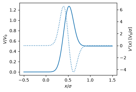
We can also do this with a gaussian and the error function if we want something analytic.
from scipy.special import erf

def V_gaussian(x, V0=0.5, sigma=2.0, dV=0.2, d=0, V0_supp=10.0):
    """Return the dth derivative of a linear potential barrier.

    Arguments
    ---------
    x : array-like
        Abscissa on which to compute the potential.
    V0 : float
        Height of barrier.
    sigma : float
        Width of barrier.
    dV : float
        Potential difference from right to left of the barrier.
    d : [0, 1]
        Derivative order.
    V0_supp : float
        The potential is shifted so that `V(0) = exp(-V_0supp)`.
    """
    s = sigma / 2
    f2 = V0_supp
    f = np.sqrt(f2)
    V0_ = V0 * np.exp(- f2 * (x / s - 1) ** 2)
    V1_ = dV * (1 + erf( f * (x / s - 1)))/2
    if d == 0:
        return V0_ + V1_
    elif d == 1:
        dV0_ = -V0 * 2 * f2 / s
        dV1_ = dV / np.sqrt(np.pi) * f / s
        return  (dV0_ * (x / s - 1) + dV1_) * np.exp(- f2 * (x / s - 1) ** 2)

V0 = 1.0
sigma = 1.0
dV = 0.5

x = sigma * np.linspace(-0.5, 1.5, 301)

V = V_gaussian(x, sigma=sigma, V0=V0, dV=dV)
dV_dx = V_gaussian(x, sigma=sigma, V0=V0, dV=dV, d=1)
assert np.allclose(np.gradient(V, x), dV_dx, rtol=0.02)

fig, ax = plt.subplots(figsize=(4, 3))
ax1 = ax.twinx()
ax.plot(x / sigma,  V / V0)
ax1.plot(x / sigma,  dV_dx / (V0/sigma), ":")

ax.set(xlabel=r"$x/\sigma$", ylabel="$V/V_0$",
       xticks=[-0.5, 0, 0.5, 1.0, 1.5])
ax1.set(ylabel=r"$V'(x)$ [$V_0/\sigma$]");